Learning to Discover Cross-Domain Relations with Generative Adversarial Networks,2017
Generative Adversarial Networks를 통해 도메인 간 관계를 발견하는 방법 배우기, 2017
Abstract
While humans easily recognize relations between data from different domains without any supervision, learning to automatically discover them is in general very challenging and needs many ground-truth pairs that illustrate the relations.
인간은 감독없이 서로 다른 도메인의 데이터 간의 관계를 쉽게 인식 할 수 있지만 자동으로 데이터를 발견하는 방법을 배우는 것은 일반적으로 매우 어렵고 관계를 설명하는 많은 근거 쌍이 필요합니다.
To avoid costly pairing, we address the task of discovering cross-domain relations given unpaired data.
값 비싼 페어링을 방지하기 위해 페어링되지 않은 데이터에서 교차 도메인 관계를 발견하는 작업을 처리합니다.
We propose a method based on generative adversarial networks that learns to discover relations between different domains (DiscoGAN). Using the discovered relations, our proposed network successfully transfers style from one domain to another while preserving key attributes such as orientation and face identity.
우리는 서로 다른 도메인 (DiscoGAN) 간의 관계를 발견하는 방법을 학습하는 생성 적 적대적 네트워크 기반 방법을 제안합니다. 발견 된 관계를 사용하여 우리가 제안한 네트워크는 방향 및 얼굴 정체성과 같은 주요 속성을 보존하면서 한 도메인에서 다른 도메인으로 스타일을 성공적으로 전송합니다.
1. Introduction
Relations between two different domains, the way in which concepts, objects, or people are connected, arise ubiquitously.
개념, 대상 또는 사람이 연결되는 방식 인 서로 다른 두 영역 간의 관계는 어디에서나 발생합니다.
Cross-domain relations are often natural to humans.
도메인 간 관계는 종종 인간에게 자연스러운 일입니다.
For example, we recognize the relationship between an English sentence and its translated sentence in French.
예를 들어, 우리는 영어 문장과 프랑스어로 번역 된 문장 사이의 관계를 인식합니다.
We also choose a suit jacket with pants or shoes in the same style to wear.
우리는 또한 같은 스타일의 바지 또는 신발이있는 정장 재킷을 선택합니다.
Can machines also achieve a similar ability to relate two different image domains?
기계가 두 개의 서로 다른 이미지 도메인을 연관시키는 유사한 기능을 달성 할 수도 있습니까?
This question can be reformulated as a conditional image generation problem.
이 질문은 조건부 이미지 생성 문제로 재구성 될 수 있습니다.
In other words, finding a mapping function from one domain to the other can be thought as generating an image in one domain given another image in the other domain.
즉, 한 도메인에서 다른 도메인으로의 매핑 함수를 찾는 것은 다른 도메인의 다른 이미지가 주어지면 한 도메인에서 이미지를 생성하는 것으로 생각할 수 있습니다
While this problem tackled by generative adversarial networks (GAN) (Isola et al., 2016) has gained a huge attention recently, most of today’s training approaches use explicitly paired data, provided by human or another algorithm.
GAN (Generative Adversarial Network) (Isola et al., 2016)에 의해 해결 된이 문제가 최근 큰 관심을 끌었지만 오늘날 대부분의 교육 접근 방식은 사람이나 다른 알고리즘이 제공하는 명시 적으로 쌍을 이룬 데이터를 사용합니다.
This problem also brings an interesting challenge from a learning point of view.
이 문제는 또한 학습 관점에서 흥미로운 도전을 가져옵니다.
Explicitly supervised data is seldom available and labeling can be labor intensive.
명시적으로 감독되는 데이터는 거의 사용할 수 없으며 라벨링은 노동 집약적 일 수 있습니다.
Moreover, pairing images can become tricky if corresponding images are missing in one domain or there are multiple best candidates.
또한 해당 이미지가 하나의 도메인에서 누락되거나 여러 최적 후보가있는 경우 이미지 페어링이 까다로울 수 있습니다
Hence, we push one step further by discovering relations between two visual domains without any explicitly paired data.
따라서 명시 적으로 쌍을 이룬 데이터없이 두 시각적 도메인 간의 관계를 발견하여 한 단계 더 나아갑니다.
In order to tackle this challenge, we introduce a model that discovers cross-domain relations with GANs (DiscoGAN).
이 문제를 해결하기 위해 GAN (DiscoGAN)과 도메인 간 관계를 발견하는 모델을 소개합니다.
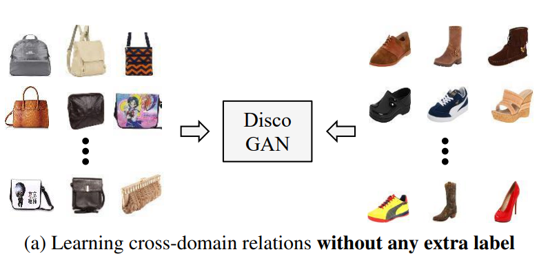
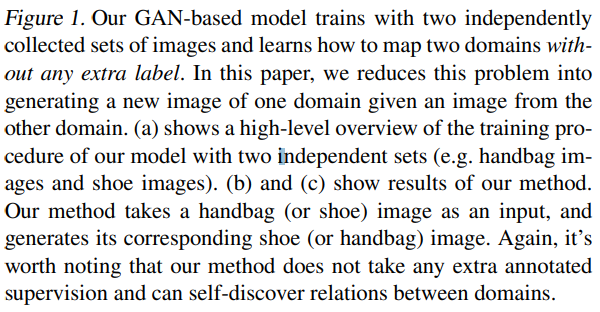
Unlike previous methods, our model can be trained with two sets of images without any explicit pair labels (see Figure 1a) and does not require any pre-training.
이전 방법과 달리 우리의 모델은 명시적인 쌍 레이블 (그림 1a 참조)없이 두 세트의 이미지로 학습 할 수 있으며 사전 학습이 필요하지 않습니다.
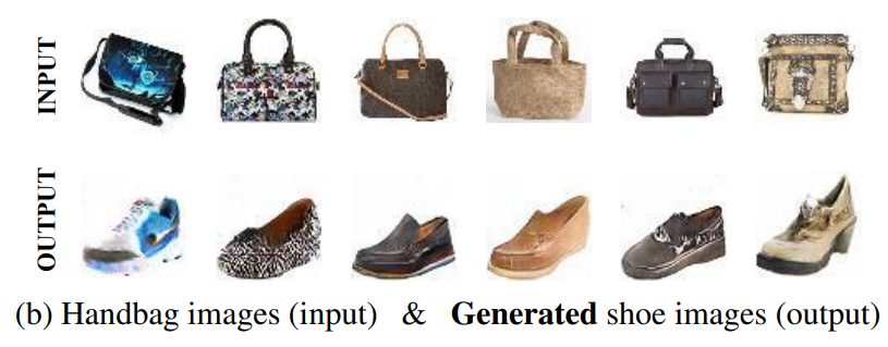
Our proposed model can then take one image in one domain as an input and generate its corresponding image in another domain (see Figure 1b).
제안 된 모델은 한 도메인에서 하나의 이미지를 입력으로 가져와 다른 도메인에서 해당 이미지를 생성 할 수 있습니다 (그림 1b 참조).
The core of our model is based on two different GANs coupled together – each of them ensures our generative functions can map each domain to its counterpart domain.
모델의 핵심은 서로 결합 된 두 개의 서로 다른 GAN을 기반으로합니다. 각 GAN은 생성 기능이 각 도메인을 해당 도메인에 매핑 할 수 있도록합니다.
A key intuition we rely on is to constraint all images in one domain to be representable by images in the other domain.
우리가 의존하는 핵심 직관은 한 도메인의 모든 이미지를 다른 도메인의 이미지로 표현할 수 있도록 제한하는 것입니다.
For example, when learning to generatea shoe image based on each handbag image, we force this generated image to be an image-based representation of the handbag image (and hence reconstruct the handbag image) through a reconstruction loss, and to be as close to images in the shoe domain as possible through a GAN loss.
예를 들어, 각 핸드백 이미지를 기반으로 신발 이미지를 생성하는 방법을 학습 할 때, 생성 된 이미지가 재구성 손실을 통해 핸드백 이미지의 이미지 기반 표현이되고 (따라서 핸드백 이미지를 재구성) GAN 손실을 통해 가능한 한 신발 도메인의 이미지.
We use these two properties to encourage the mapping between two domains to be well covered on both directions (i.e. encouraging one-to-one rather than many-to-one or one-tomany). In the experimental section, we show that this simple intuition discovered common properties and styles of two domains very well.
이 두 가지 속성을 사용하여 두 도메인 간의 매핑이 양방향에서 잘 다루어 지도록 장려합니다 (예 : 다 대일 또는 일대일보다는 일대일 권장).
Both experiments on toy domain and real world image datasets support the claim that our proposed model is wellsuited for discovering cross-domain relations.
험 섹션에서 우리는이 단순한 직관이 두 영역의 공통 속성과 스타일을 아주 잘 발견했음을 보여줍니다.
When translating data points between simple 2-dimensional domains and between face image domains, our DiscoGAN model was more robust to the mode collapse problem compared to two other baseline models.
장난감 도메인과 실제 이미지 데이터 세트에 대한 실험 모두 우리가 제안한 모델이 교차 도메인 관계를 발견하는 데 적합하다는 주장을 뒷받침합니다.
It also learns the bidirectional mapping between two image domains, such as faces, cars, chairs, edges and photos, and successfully apply them in image translation.
또한 얼굴, 자동차, 의자, 가장자리 및 사진과 같은 두 이미지 도메인 간의 양방향 매핑을 학습하고 이미지 번역에 성공적으로 적용합니다.
Translated images consistently change specified attributes such as hair color, gender and orientation while maintaining all other components.
번역 된 이미지는 다른 모든 구성 요소를 유지하면서 머리 색깔, 성별 및 방향과 같은 지정된 속성을 지속적으로 변경합니다.
Results also show that our model is robust to repeated application of translation mappings.
결과는 또한 우리 모델이 번역 매핑을 반복적으로 적용 할 수 있다는 것을 보여줍니다.
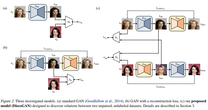
그림 2. 세 가지 조사 된 모델. (a) 표준 GAN (Goodfellow et al., 2014), (b) 재구성 손실이있는
2. Model
We now formally define cross-domain relations and present the problem of learning to discover such relations in two different domains.
이제 우리는 공식적으로 교차 도메인 관계를 정의하고 두 개의 다른 도메인에서 그러한 관계를 발견하는 방법을 배우는 문제를 제시합니다.
Standard GAN model and a similar variant model with additional components are investigated for their applicability for this task.
표준 GAN 모델 및 추가 구성 요소가있는 유사한 변형 모델이 이 작업에 대한 적용 가능성을 조사합니다.
Limitations of these models are then explained, and we propose a new architecture based on GANs that can be used to discover cross-domain relations.
그런 다음 이러한 모델의 한계를 설명하고 도메인 간 관계를 발견하는 데 사용할 수있는 GAN 기반의 새로운 아키텍처를 제안합니다.
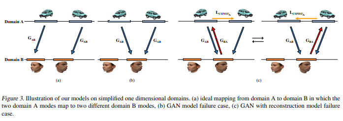
그림 3. 단순화 된 1 차원 도메인에 대한 모델 그림. (a) 도메인 A에서 도메인 B 로의 이상적인 매핑 두 개의 도메인 A 모드는 두 개의 다른 도메인 B 모드에 매핑됩니다. (b) GAN 모델 실패 사례, (c) 재구성 모델 실패가있는 GAN 케이스.
2.1. Formulation
Relation is mathematically defined as a function GAB that maps elements from its domain A to elements in its codomain B and GBA is similarly defined.
관계는 수학적으로 도메인 A의 요소를 공동 도메인 B의 요소에 매핑하는 함수 GAB로 정의되며 GBA는 유사하게 정의됩니다.
In fully unsupervised setting, GAB and GBA can be arbitrarily defined.
완전 비 감독 설정에서는 GAB와 GBA를 임의로 정의 할 수 있습니다.
To find a meaningful relation, we need to impose a condition on the relation of interest.
의미있는 관계를 찾으려면 관심 관계에 조건을 부여해야합니다.
Here, we constrain relation to be a one-to-one correspondence (bijective mapping).
여기서는 관계를 일대일 대응 (용사 매핑)으로 제한합니다
That means GAB is the inverse mapping of GBA.
즉, GAB는 GBA의 역 매핑입니다.
The range of function GAB, the complete set of all possible resulting values GAB(xA) for all xA’s in domain A, should be contained in domain B and similarly for GBA(xB).
도메인 A의 모든 xA에 대해 가능한 모든 결과 값 GAB (xA)의 전체 집합 인 함수 GAB의 범위는 도메인 B에 포함되어야하며 마찬가지로 GBA (xB)에 대해서도 포함되어야합니다.
We now relate these constraints to objective functions.
이제 이러한 제약을 목적 함수와 관련시킵니다.
Ideally, the equality GBA ◦ GAB(xA) = xA should be satisfied, but this hard constraint is difficult to optimize and relaxed soft constraint is more desirable in the view of optimization.
이상적으로는 동등성 GBA ◦ GAB (xA) = xA를 충족해야하지만이 하드 제약 조건은 최적화하기 어렵고 최적화 관점에서 완화 된 소프트 제약 조건이 더 바람직합니다.
For this reason, we minimize the distance d(GBA ◦ GAB(xA), xA), where any form of metric function (L1, L2, Huber loss) can be used.
따라서 모든 형태의 미터법 함수 (L1, L2, Huber 손실)를 사용할 수있는 거리 d (GBA ◦ GAB (xA), xA)를 최소화합니다.
Similarly, we also need to minimize d(GAB ◦ GBA(xB), xB).
마찬가지로 d (GAB ◦ GBA (xB), xB)도 최소화해야합니다.
Guaranteeing that GAB maps to domain B is also very difficult to optimize.
GAB가 도메인 B에 매핑되도록 보장하는 것도 최적화하기 매우 어렵습니다.
We relax this constraint as follows: we instead minimize generative adversarial loss −ExA ∼PA[log DB(GAB(xA ))].
이 제약을 다음과 같이 완화합니다. 대신 생성 적대 손실 −ExA ∼PA [log DB (GAB (xA))]를 최소화합니다
Similarly, we minimize−ExB ∼PB[log DA(GBA(xB ))].
마찬가지로 ExB ~ PB [log DA (GBA (xB))]를 최소화합니다.
Now, we explore several GAN architectures to learn with these loss functions.
이제 우리는 이러한 손실 함수를 배우기 위해 몇 가지 GAN 아키텍처를 탐색합니다.
2.2. Notation and Architecture
We use the following notations in sections below.
아래 섹션에서 다음 표기법을 사용합니다.
A generator network is denoted GAB : R64×64×3A → R 64×64×3B , and the subscripts denote the input and output domains and superscripts denote the input and output image size.
생성기 네트워크는 GAB : R64 × 64 × 3A → R 64 × 64 × 3B로 표시되고 아래 첨자는 입력 및 출력 도메인을 나타내고 위 첨자는 입력 및 출력 이미지 크기를 나타냅니다.
The discriminator network is denoted as DB : R64×64×3B → [0, 1],and the subscript B denotes that it discriminates images in domain B. Notations GBA and DA are used similarly.
판별 기 네트워크는 DB : R64 × 64 × 3B → [0, 1]로 표시하고, 아래 첨자 B는 도메인 B에서 이미지를 판별 함을 나타냅니다. 표기법 GBA와 DA는 유사하게 사용됩니다
Each generator takes image of size 64×64×3 and feeds it through an encoder-decoder pair.
각 생성기는 64x64x3 크기의 이미지를 가져 와서 인코더-디코더 쌍을 통해 공급합니다.
The encoder part of each generator is composed of convolution layers with 4 × 4 filters, each followed by leaky ReLU (Maas et al., 2013; Xuet al., 2015).
각 생성기의 인코더 부분은 4 × 4 필터가있는 컨볼 루션 레이어로 구성되며 각 필터는 누수 ReLU가 뒤 따릅니다 (Maas et al., 2013; Xuet al., 2015).
The decoder part is composed of deconvolution layers with 4 × 4 filters, followed by a ReLU, and outputs a target domain image of size 64×64×3.
디코더 부분은 4 × 4 필터와 ReLU가 뒤 따르는 디콘 볼 루션 레이어로 구성되어 있으며 64 × 64 × 3 크기의 타겟 도메인 이미지를 출력합니다.
The number of convolution and deconvolution layers ranges from four to five, depending on the domain.
컨볼 루션 및 디컨 볼 루션 레이어의 수는 도메인에 따라 4 ~ 5 개입니다.
The discriminator is similar to the encoder part of the generator.
판별 기는 생성기의 인코더 부분과 유사합니다.
In addition to the convolution layers and leaky ReLUs, the discriminator has an additional convolution layer with 4 × 4 filters, and a final sigmoid to output a scalar output between [0, 1].
컨볼 루션 레이어 및 누출 ReLU 외에도 판별 기는 4 × 4 필터가있는 추가 컨볼 루션 레이어와 [0, 1] 사이의 스칼라 출력을 출력하는 최종 시그 모이 드를 갖습니다.
2.3. GAN with a Reconstruction Loss
We first consider a standard GAN model (Goodfellow et al., 2014) for the relation discovery task (Figure 2a).
먼저 관계 검색 작업을위한 표준 GAN 모델 (Goodfellow et al., 2014)을 고려합니다 (그림 2a).
Originally, a standard GAN takes random Gaussian noise z, encodes it into hidden features h and generates images such as MNIST digits.
원래 표준 GAN은 임의의 가우스 노이즈 z를 가져 와서 숨겨진 특징 h로 인코딩하고 MNIST 숫자와 같은 이미지를 생성합니다.
We make a slight modification to this model to fit our task: the model we use takes in image as input instead of noise.
작업에 맞게이 모델을 약간 수정합니다. 사용하는 모델은 노이즈 대신 이미지를 입력으로 사용합니다.
In addition, since this architecture only learns one mapping from domain A to domain B, we add a second generator that maps domain B back into domain A (Figure 2b).
또한이 아키텍처는 도메인 A에서 도메인 B 로의 매핑을 하나만 학습하므로 도메인 B를 다시 도메인 A로 매핑하는 두 번째 생성기를 추가합니다 (그림 2b).
We also add a reconstruction loss term that compares the input image with the reconstructed image.
또한 입력 이미지와 재구성 된 이미지를 비교하는 재구성 손실 항을 추가합니다.
With these additional changes, each generator in the model can learn mapping from its input domain to output domain and discover relations between them.
이러한 추가 변경으로 모델의 각 생성기는 입력 도메인에서 출력 도메인으로의 매핑을 학습하고 이들 간의 관계를 발견 할 수 있습니다
A generator GAB translates input image xA from domain A into xAB in domain B.
생성기 GAB는 입력 이미지 xA를 도메인 A에서 도메인 B의 xAB로 변환합니다
The generated image is then translated into a domain A image xABA to match the original input image (Equation 1, 2).
생성 된 이미지는 원본 입력 이미지와 일치하도록 도메인 A 이미지 xABA로 변환됩니다 (수식 1, 2).
Various forms of distance functions, such as MSE, cosine distance, and hinge-loss, can be used as the reconstruction loss d (Equation 3).
MSE, 코사인 거리, 힌지 손실과 같은 다양한 형태의 거리 함수를 재구성 손실 d로 사용할 수 있습니다 (수식 3).
The translated output xAB is then scored by the discriminator which compares it to a real domain B sample xB.
번역 된 출력 xAB는 실제 도메인 B 샘플 xB와 비교하는 판별기에 의해 점수가 매겨집니다.
The generator GAB receives two types of losses – a reconstruction loss LCONSTA(Equation 3) that measures how well the original input is reconstructed after a sequence of two generations, and a standard GAN generator loss LGANB (Equation 4) that measures how realistic the generated image is in domain B.
생성기 GAB는 두 가지 유형의 손실을 수신합니다. 두 가지 유형의 손실은 두 세대의 시퀀스 후에 원래 입력이 얼마나 잘 재구성되는지를 측정하는 재구성 손실 LCONSTA (수식 3)와 생성 된 것이 얼마나 현실적인지를 측정하는 표준 GAN 생성기 손실 LGANB (수식 4)입니다. 이미지가 도메인 B에 있습니다.
The discriminator receives the standard GAN discriminator loss of Equation 6.
판별자는 방정식 6의 표준 GAN 판별 기 손실을받습니다.
During training, the generator GAB learns the mapping from domain A to domain B under two relaxed constraints: that domain A maps to domain B, and that the mapping on domain B is reconstructed to domain A.
훈련 중에 생성기 GAB는 두 가지 완화 된 제약 조건 하에서 도메인 A에서 도메인 B 로의 매핑을 학습합니다. 해당 도메인 A는 도메인 B에 매핑되고 도메인 B의 매핑은 도메인 A로 재구성됩니다.
However, this model lacks a constraint on mapping from B to A, and these two conditions alone does not guarantee a cross-domain relation (as defined in section 2.1) because the mapping satisfying these constraints is one-directional.
그러나이 모델에는 B에서 A 로의 매핑에 대한 제약이 없으며, 이러한 제약을 충족하는 매핑이 단방향이기 때문에이 두 조건만으로는 도메인 간 관계 (섹션 2.1에 정의 됨)를 보장하지 않습니다.
In other words, the mapping is an injection, not bijection, and one-to-one correspondence is not guaranteed.
즉, 매핑은 bijection이 아닌 주입이며 일대일 대응이 보장되지 않습니다.
Consider the two possibly multi-modal image domains A and B.
두 가지 가능한 다중 모달 이미지 도메인 A와 B를 고려하십시오.
Figure 3 illustrates the two multi-modal data domains on a simplified one-dimensional representation.
그림 3은 단순화 된 1 차원 표현에 대한 두 개의 다중 모달 데이터 도메인을 보여줍니다.
Figure 3a shows the ideal mapping from input domain A to domain B, where each mode of data is mapped to a separate mode in the target domain.
그림 3a는 입력 도메인 A에서 도메인 B 로의 이상적인 매핑을 보여줍니다. 여기서 각 데이터 모드는 대상 도메인의 개별 모드에 매핑됩니다.
Figure 3b, in contrast, shows the mode collapse problem, a prevalent phenomenon in GANs, where data from multiple modes of a domain map to a single mode of a different domain.
대조적으로, 그림 3b는 GAN에서 널리 퍼진 현상 인 모드 붕괴 문제를 보여줍니다. 여기서 도메인의 여러 모드의 데이터가 다른 도메인의 단일 모드에 매핑됩니다.
For instance, this case is where the mapping GAB maps images of cars in two different orientations into the same mode of face images.
예를 들어,이 경우 매핑 GAB는 서로 다른 두 방향의 자동차 이미지를 동일한 얼굴 이미지 모드로 매핑합니다.
In some sense, the addition of a reconstruction loss to a standard GAN is an attempt to remedy the mode collapse problem.
어떤 의미에서 표준 GAN에 재구성 손실을 추가하는 것은 모드 붕괴 문제를 해결하려는 시도입니다.
In Figure 3c, two domain A modes are matched with the same domain B mode, but the domain B mode can only direct to one of the two domain A modes.
그림 3c에서 두 도메인 A 모드는 동일한 도메인 B 모드와 일치하지만 도메인 B 모드는 두 도메인 A 모드 중 하나로 만 지정할 수 있습니다.
Although the additional reconstruction loss LCONSTA forces the reconstructed sample to match the original (Figure 3c), this change only leads to a similar symmetric problem.
추가 재구성 손실 LCONSTA는 재구성 된 샘플이 원본과 일치하도록 강제하지만 (그림 3c),이 변경으로 인해 유사한 대칭 문제가 발생합니다.
The reconstruction loss leads to an oscillation between the two states and does not resolve mode-collapsing.
재구성 손실은 두 상태 사이의 진동으로 이어지며 모드 붕괴를 해결하지 않습니다.
2.4. Our Proposed Model: Discovery GAN
Our proposed GAN model for relation discovery – DiscoGAN – couples the previously proposed model (Figure 2c).
관계 발견을 위해 제안 된 GAN 모델 인 DiscoGAN은 이전에 제안 된 모델을 결합합니다 (그림 2c).
Each of the two coupled models learns the mapping from one domain to another, and also the reverse mapping to for reconstruction.
두 결합 모델 각각은 한 도메인에서 다른 도메인으로의 매핑과 재구성을위한 역 매핑을 학습합니다.
The two models are trained together simultaneously.
두 모델은 동시에 함께 훈련됩니다
The two generators GAB’s and the two generators GBA’s share parameters, and the generated images xBA and xAB are each fed into separate discriminators LDA and LDB , respectively.
두 생성기 GAB 및 두 생성기 GBA는 매개 변수를 공유하고 생성 된 이미지 xBA 및 xAB는 각각 별도의 식별기 LDA 및 LDB에 공급됩니다.
One key difference from the previous model is that input images from both domains are reconstructed and that there are two reconstruction losses: LCONSTA and LCONSTB .
이전 모델과의 한 가지 주요 차이점은 두 도메인의 입력 이미지가 재구성되고 LCONSTA 및 LCONSTB의 두 가지 재구성 손실이 있다는 것입니다.
As a result of coupling two models, the total generator loss is the sum of GAN loss and reconstruction loss for each partial model (Equation 7).
두 모델을 결합한 결과 총 발전기 손실은 각 부분 모델에 대한 GAN 손실과 재구성 손실의 합입니다 (수식 7
Similarly, the total discriminator loss LD is a sum of discriminator loss for the two discriminators DA and DB, which discriminate real and fake images of domain A and domain B (Equation 8).
마찬가지로 총 판별 기 손실 LD는 두 판별 기 DA 및 DB에 대한 판별 기 손실의 합으로, 도메인 A와 도메인 B의 실제 이미지와 가짜 이미지를 구별합니다 (수식 8).
Now, this model is constrained by two LGAN losses and two LCONST losses.
이제 이 모델은 2 개의 LGAN 손실과 2 개의 LCONST 손실로 제한됩니다.
Therefore a bijective mapping is achieved, and a one-to-one correspondence, which we defined as cross-domain relation, can be discovered.
따라서 bijective 매핑이 이루어지고 도메인 간 관계로 정의한 일대일 대응이 발견 될 수 있습니다.
3. Experiments
3.1. Toy Experiment

그림 4. 장난감 도메인 실험 결과. 컬러 배경은 판별 기의 출력 값을 보여줍니다. 'x'표시는 다른 것을 나타냅니다. B 도메인의 모드와 색칠 된 원은 도메인 A에서 도메인 B에 매핑 된 샘플을 나타내며, 여기서 각 색상은 서로 다른 방법. (a) 10 개의 대상 도메인 모드 및 초기 번역, (b) 표준 GAN 모델, (c) 재구성 손실이있는 GAN, (d) 제안 된
To empirically demonstrate our explanations on the differences between a standard GAN, a GAN with reconstruction loss and our proposed model (DiscoGAN), we designed an illustrative experiment based on synthetic data in 2-dimensional A and B domains.
표준 GAN, 재구성 손실이있는 GAN 및 제안 된 모델 (DiscoGAN) 간의 차이점에 대한 설명을 실증적으로 설명하기 위해 2 차원 A 및 B 도메인의 합성 데이터를 기반으로 한 실례 실험을 설계했습니다.
Both source and target data samples are drawn from Gaussian mixture models.
소스 및 대상 데이터 샘플은 모두 가우스 혼합 모델에서 가져옵니다.
In Figure 4, the left-most figure shows the initial state of toy experiment where all the A domain modes map to almost a single point because of initialization of the generator.
그림 4에서 가장 왼쪽 그림은 생성기 초기화로 인해 모든 A 도메인 모드가 거의 단일 지점에 매핑되는 장난감 실험의 초기 상태를 보여줍니다.
For all other plots the target domain 2D plane is shown with target domain modes marked with black ‘x’s.
다른 모든 플롯의 경우 대상 도메인 2D 평면이 검은 색 'x'로 표시된 대상 도메인 모드로 표시됩니다.
Colored points on B domain planes represent samples from A domain that are mapped to the B domain, and each color denotes samples from each A domain mode.
B 도메인 평면의 컬러 포인트는 B 도메인에 매핑 된 A 도메인의 샘플을 나타내고 각 색상은 각 A 도메인 모드의 샘플을 나타냅니다.
In this case, the task is to discover cross-domain relations between the A and B domain and translate samples from five A domain modes into the B domain, which has ten modes spread around the arc of a circle.
이 경우 작업은 A와 B 도메인 간의 교차 도메인 관계를 발견하고 5 개의 A 도메인 모드의 샘플을 원호 주위에 10 개의 모드가 분산 된 B 도메인으로 변환하는 것입니다.
We use a neural network with three linear layers that are each followed by a ReLU nonlinearity as the generator.
우리는 각각 ReLU 비선형 성이 생성기로 뒤 따르는 3 개의 선형 계층이있는 신경망을 사용합니다.
For the discriminator we use five linear layers that are each followed by a ReLU, except for the last layer which is switched out with a sigmoid that outputs a scalar ∈ [0, 1].
판별기의 경우 스칼라 ∈ [0, 1]을 출력하는 시그 모이 드로 전환 된 마지막 계층을 제외하고 각각 뒤에 ReLU가 오는 5 개의 선형 계층을 사용합니다
The colored background shows the output value of the discriminator DB, which discriminates real target domain samples from synthetic, translated samples from domain A.
컬러 배경은 도메인 A의 합성, 번역 된 샘플에서 실제 대상 도메인 샘플을 구별하는 판별 기 DB의 출력 값을 보여줍니다.
The contour lines show regions of same discriminator value.
등고선은 동일한 판별 기 값의 영역을 보여줍니다.
The training was performed for 50,000 iterations, and due to the domain simplicity our model often converged much earlier.
훈련은 50,000 번의 반복으로 수행되었으며 도메인 단순성으로 인해 우리 모델은 종종 훨씬 일찍 수렴되었습니다.
The results from this experiment match our claim and illustrations in Figure 4 and the resulting translated samples show very different behavior depending on the model used.
이 실험의 결과는 우리의 주장과 그림 4의 삽화와 일치하며 결과로 번역 된 샘플은 사용 된 모델에 따라 매우 다른 동작을 보여줍니다.
In the baseline (standard GAN) case, many translated points of different colors are located around the same B domain mode.
기준선 (표준 GAN)의 경우 서로 다른 색상으로 변환 된 많은 포인트가 동일한 B 도메인 모드 주변에 위치합니다.
For example, navy and light-blue colored points are located together, as well as green and orange colored points.
예를 들어, 네이비 및 라이트 블루 색상의 포인트와 녹색 및 주황색 포인트가 함께 위치합니다.
This result illustrates the mode-collapse problem of GANs since points of multiple colors (multiple A domain modes) are mapped to the same B domain mode.
이 결과는 여러 색상의 포인트 (다중 A 도메인 모드)가 동일한 B 도메인 모드에 매핑되기 때문에 GAN의 모드 붕괴 문제를 보여줍니다.
The baseline model still oscillate around B modes throughout the iterations.
기준 모델은 반복하는 동안 B 모드를 중심으로 여전히 진동합니다.
In the case of GAN with a reconstruction loss, the collapsing problem is less prevalent, but navy, green and light-blue points still overlap at a few modes.
재구성 손실이있는 GAN의 경우 붕괴 문제가 덜 발생하지만 해군, 녹색 및 하늘색 점은 여전히 몇 가지 모드에서 겹칩니다.
The contour plot also demonstrates the difference from baseline: regions around all B modes are leveled in a green colored plateau in the baseline, allowing translated samples to freely move between modes, whereas in the single model case the regions between B modes are clearly separated.
등고선 플롯은 또한 기준선과의 차이를 보여줍니다. 모든 B 모드 주변 영역은 기준선에서 녹색 고원으로 평평 해져 변환 된 샘플이 모드간에 자유롭게 이동할 수있는 반면 단일 모델의 경우 B 모드 간의 영역이 명확하게 분리됩니다.
In addition, both this model and the standard GAN model fail to cover all modes in B domain since the mapping from A domain to B domain is injective. Our proposed DiscoGAN model, on the other hand, is able to not only prevent mode-collapse by translating into distinct well-bounded regions that do not overlap, but also generate B samples in all ten modes as the mappings in our model is bijective.
또한, 이 모델과 표준 GAN 모델은 A 도메인에서 B 도메인으로의 매핑이 주입 적이므로 B 도메인의 모든 모드를 포함하지 못합니다. 반면에 우리가 제안한 DiscoGAN 모델은 겹치지 않는 고유 한 경계 영역으로 변환하여 모드 붕괴를 방지 할 수있을뿐만 아니라 모델의 매핑이 bijective이므로 10 개 모드 모두에서 B 샘플을 생성 할 수 있습니다.
It is noticeable that the discriminator for B domain is perfectly fooled by translated samples from A domain around B domain modes.
B 도메인의 판별자는 B 도메인 모드를 중심으로 A 도메인에서 번역 된 샘플에 완벽하게 속는다는 것이 눈에 띕니다
Although this experiment is limited due to its simplicity, the results clearly support the superiority of our proposed model over other variants of GANs.
이 실험은 단순성으로 인해 제한적이지만 결과는 제안 된 모델이 다른 GAN 변형보다 우월함을 분명히 뒷받침합니다.
3.2. Real Domain Experiment
To evaluate whether our DiscoGAN successfully learns underlying relationship between domains, we trained and tested our model using several image-to-image translation tasks that require the use of discovered cross-domain relations between source and target domains.
DiscoGAN이 도메인 간의 기본 관계를 성공적으로 학습했는지 평가하기 위해 소스 및 대상 도메인 간의 발견 된 도메인 간 관계를 사용해야하는 여러 이미지 대 이미지 변환 작업을 사용하여 모델을 훈련하고 테스트했습니다.
In each real domain experiment, all input images and translated images were of size 64 × 64 × 3.
각 실제 도메인 실험에서 모든 입력 이미지와 번역 된 이미지의 크기는 64 × 64 × 3입니다.
For training, we used learning rate of 0.0002 and used the Adam optimizer (Kingma & Ba, 2015) with β1 = 0.5 and β2 = 0.999.
훈련을 위해 0.0002의 학습률을 사용하고 β1 = 0.5 및 β2 = 0.999 인 Adam 최적화 프로그램 (Kingma & Ba, 2015)을 사용했습니다.
We applied Batch Normalization (Ioffe & Szegedy, 2015) to all convolution and deconvolution layers except the first and the last layers, weight decay regularization coefficient of 10−4 and minibatch of size 200.
배치 정규화 (Ioffe & Szegedy, 2015)를 첫 번째 및 마지막 레이어를 제외한 모든 컨볼 루션 및 디컨 볼 루션 레이어, 가중치 감쇠 정규화 계수 10-4 및 크기 200의 미니 배치에 적용했습니다.
All computations were conducted on a single machine with an Nvidia Titan X Pascal GPU and an Intel(R) Xeon(R) E5-1620 CPU.
모든 계산은 Nvidia Titan X Pascal GPU와 Intel (R) Xeon (R) E5-1620 CPU가 장착 된 단일 시스템에서 수행되었습니다.
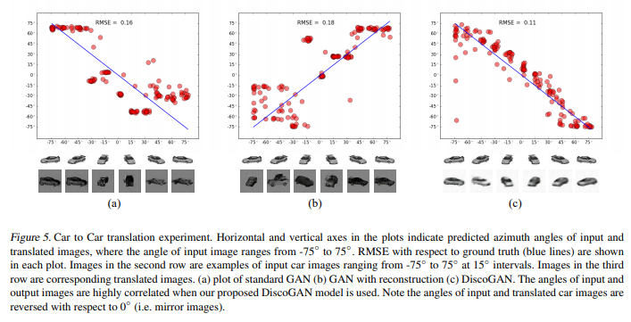
그림 5. Car to Car 번역 실험. 플롯의 수평 및 수직 축은 예측 된 방위각 입력 및 변환 된 이미지, 입력 이미지의 각도 범위는 -75 °입니다. ~ 75◦ . Ground Truth (파란색 선)에 대한 RMSE가 표시됩니다. 각 줄거리에서. 두 번째 행의 이미지는 -75o 범위의 입력 차량 이미지의 예입니다. ~ 75◦ 15◦에 간격. 세 번째 이미지 행은 해당 번역 이미지입니다. (a) 표준 GAN 플롯 (b) 재구성 된 GAN (c) DiscoGAN. 입력 각도와 출력 이미지는 소품이
3.2.1. CAR TO CAR, FACE TO FACE
We used a Car dataset (Fidler et al., 2012) which consists of rendered images of 3D car models with varying azimuth angles at 15◦intervals.
우리는 15o 간격에서 다양한 방위각을 가진 3D 자동차 모델의 렌더링 된 이미지로 구성된 Car 데이터 세트 (Fidler et al., 2012)를 사용했습니다.
We split the dataset into train and test sets and again split the train set into two groups, each of which is used as A domain and B domain samples.
데이터 세트를 학습 세트와 테스트 세트로 분할하고 학습 세트를 다시 두 그룹으로 분할했습니다. 각 그룹은 A 도메인과 B 도메인 샘플로 사용됩니다.
In addition to training a standard GAN model, a GAN with a reconstruction model and a proposed DiscoGAN model, we also trained a regressor that predicts the azimuth angle of a car image using the train set.
표준 GAN 모델, 재구성 모델이있는 GAN 및 제안 된 DiscoGAN 모델을 학습하는 것 외에도 기차 세트를 사용하여 자동차 이미지의 방위각을 예측하는 회귀자를 학습했습니다.
To evaluate, we translated images in the test set using each of the three trained models, and azimuth angles were predicted using the regressor for both input and translated images.
평가하기 위해 세 가지 훈련 된 모델 각각을 사용하여 테스트 세트의 이미지를 번역하고 입력 이미지와 번역 이미지 모두에 대해 회귀자를 사용하여 방위각을 예측했습니다.
Figure 5 shows the predicted azimuth angles of input and translated images for each model.
그림 5는 각 모델에 대한 입력 및 변환 된 이미지의 예측 방위각을 보여줍니다.
In standard GAN and GAN with reconstruction (5a and 5b), most of the red dots are grouped in a few clusters, indicating that most of the input images are translated into images with same azimuth, and that these models suffer from mode collapsing problem as predicted and shown in Figures 3 and 4.
재구성 된 표준 GAN 및 GAN (5a 및 5b)에서 대부분의 빨간색 점은 몇 개의 클러스터로 그룹화되어 대부분의 입력 이미지가 동일한 방위각을 가진 이미지로 변환되고 이러한 모델은 다음과 같은 모드 축소 문제가 있음을 나타냅니다. 예측되고 그림 3과 4에 나와 있습니다.
Our proposed DiscoGAN (5c), on the other hand, shows strong correlation between predicted angles of input and translated images, indicating that our model successfully discovers azimuth relation between the two domains.
반면에 우리가 제안한 DiscoGAN (5c)은 예측 된 입력 각도와 번역 된 이미지 사이에 강한 상관 관계를 보여 주어 우리 모델이 두 도메인 간의 방위각 관계를 성공적으로 발견했음을 나타냅니다.
In this experiment, the translated images either have the same azimuth range (5b), or the opposite (5a and 5c) of the input images.
이 실험에서 번역 된 이미지는 동일한 방위각 범위 (5b)를 갖거나 입력 이미지의 반대 (5a 및 5c)를 갖습니다.
Next, we use a Face dataset (Paysan et al., 2009) shown in Figure 6a, in which the data images vary in azimuth rotation from -90◦to +90◦.
다음으로 그림 6a에 표시된 Face 데이터 세트 (Paysan et al., 2009)를 사용합니다. 여기서 데이터 이미지는 -90o에서 + 90o까지 방위각 회전이 다릅니다.
Similar to previous car to car experiment, input images in the -90◦to +90◦rotation range generated output images either in the same range, from -90◦to+90◦, or the opposite range, from +90◦to -90◦ when our proposed model was used (6d).
이전의 자동차 대 자동차 실험과 유사하게 -90o에서 + 90o 회전 범위의 입력 이미지는 -90o에서 + 90o 사이의 동일한 범위 또는 + 90o에서 + 90o 사이의 반대 범위에서 출력 이미지를 생성했습니다. 90◦ 제안 된 모델이 사용되었을 때 (6d). 또한 비교를 위해 재구성 손실이있는 표준 GAN 및 GAN을 훈련했습니다
We also trained a standard GAN and a GAN with reconstruction loss for comparison.
또한 비교를 위해 재구성 손실이있는 표준 GAN 및 GAN을 훈련했습니다.
When a standard GAN and GAN with reconstruction loss were used, the generated images do not vary as much as the input images in terms of rotation.
재구성 손실이있는 표준 GAN 및 GAN을 사용하면 생성 된 이미지가 회전 측면에서 입력 이미지만큼 변하지 않습니다.
In this sense, similar to what has been shown in previous Car to Car experiment, the two models suffered from mode collapse.
이러한 의미에서 이전 Car to Car 실험에서 보여준 것과 유사하게 두 모델은 모드 붕괴를 겪었습니다.
3.2.2. FACE CONVERSION
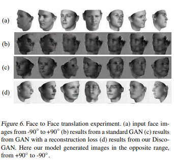
그림 6. 대면 번역 실험. (a) -90◦에서 입력 얼굴 이미지 ~ + 90◦ (b) 표준 GAN의 결과 (c) 결과 재구성 손실 (d)이있는 GAN의 결과는 DiscoGAN의 결과입니다. 여기서 우리 모델은 반대 범위에서 이미지를 생성했습니다. + 90◦에서 ~ -90◦
In terms of the amount of related information between two domains, we can consider a few extreme cases: two domains sharing almost all features and two domains sharing only one feature.
두 도메인 간의 관련 정보 양 측면에서 몇 가지 극단적 인 경우를 고려할 수 있습니다. 두 도메인은 거의 모든 기능을 공유하고 두 도메인은 하나의 기능 만 공유합니다.
To investigate former case, we applied the face attribute conversion task on CelebA dataset (Liu et al., 2015), where only one feature, such as gender or hair color, varies between two domains and all the other facial features are shared.
이전 사례를 조사하기 위해 CelebA 데이터 세트 (Liu et al., 2015)에 얼굴 속성 변환 작업을 적용했습니다. 여기서 성별 또는 머리 색깔과 같은 하나의 특징 만 두 도메인간에 다르며 다른 모든 얼굴 특징은 공유됩니다.
The results are listed in Figure 7.
결과는 그림 7에 나와 있습니다.
In Figure 7a, we can see that various facial features are well-preserved while a single desired attribute (gender) is changed.
그림 7a에서 원하는 단일 속성 (성별)이 변경되는 동안 다양한 얼굴 특징이 잘 보존되어 있음을 알 수 있습니다.
Also, 7b and 7d shows that background is also well-preserved and images are visually natural, although the background does change in a few cases such as Figure 7c.
또한 7b와 7d는 그림 7c와 같은 일부 경우 배경이 변경되지만 배경도 잘 보존되어 있고 이미지가 시각적으로 자연 스럽다는 것을 보여줍니다.
An extension to this experiment was sequentially applying several translations – for example, changing the gender and then the hair color (7e), or repeatedly applying gender transforms (7f).
이 실험의 확장은 몇 가지 번역을 순차적으로 적용하는 것이 었습니다. 예를 들어 성별을 변경 한 다음 머리 색깔을 변경하거나 (7e), 성별 변환을 반복적으로 적용 (7f)하는 것입니다
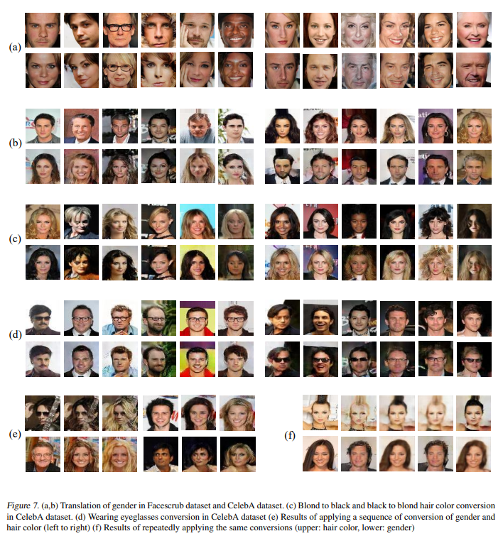
그림 7. (a, b) Facescrub 데이터 셋과 CelebA 데이터 셋에서 성별 번역. (c) 금발에서 검은 색으로, 검은 색에서 금발 머리로 색상 변환 CelebA 데이터 셋에서. (d) CelebA 데이터 세트에서 안경 착용 변환 (e) 성별 및 성별 변환 시퀀스를 적용한 결과 머리 색 (왼쪽에서 오른쪽으로) (f) 동일한 변환을 반복적으로 적용한 결과 (상단 : 머리 색, 하단 : 성별)
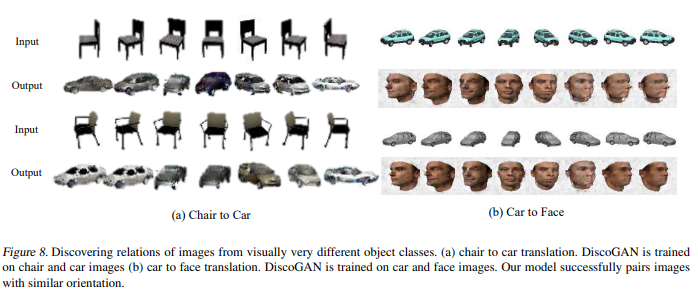
그림 8. 시각적으로 매우 다른 객체 클래스에서 이미지의 관계 발견. (a) 의자에서 자동차로의 번역. DiscoGAN은 교육을 받았습니다. 의자 및 자동차 이미지 (b) 자동차 대면 번역. DiscoGAN은 자동차 및 얼굴 이미지에 대한 교육을 받았습니다. 우리 모델은 성공적으로 이미지를 짝짓습니다. 비슷한 방향으로.
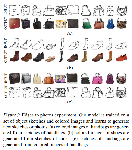
그림 9. 사진 실험에 가장자리. 우리 모델은 개체 스케치 및 컬러 이미지 세트를 생성하고 새로운 스케치 또는 사진. (a) 핸드백 스케치에서 핸드백의 컬러 이미지를 생성하고, (b) 신발의 컬러 이미지는 신발 스케치에서 생성 된, (c) 핸드백 스케치는 핸드백의 컬러 이미지에서 생성
3.2.3. CHAIR TO CAR, CAR TO FACE
We also investigated the opposite case where there is a single shared feature between two domains.
또한 두 도메인간에 단일 공유 기능이있는 반대 사례도 조사했습니다.
3D rendered images of chair (Aubry et al., 2014) and the previously used car and face datasets (Fidler et al., 2012; Paysan et al.,2009) were used in this task.
의자의 3D 렌더링 이미지 (Aubry et al., 2014)와 이전에 사용 된 자동차 및 얼굴 데이터 세트 (Fidler et al., 2012; Paysan et al., 2009)가이 작업에 사용되었습니다.
All three datasets vary along the azimuth rotation.
세 가지 데이터 세트는 모두 방위각 회전을 따라 다릅니다
Figure 8 shows the results of imageto-image translation from chair to car and from car to face datasets.
그림 8은 의자에서 자동차로, 자동차에서 얼굴로 이미지를 이미지로 변환 한 결과를 보여줍니다.
The translated images clearly match the rotation feature of the input images while preserving visual features of car and face domain, respectively.
번역 된 이미지는 입력 이미지의 회전 특성과 명확하게 일치하는 동시에 자동차 및 얼굴 도메인의 시각적 특성을 각각 유지합니다.
3.2.4. EDGES-TO-PHOTOS
Edges-to-photos is an interesting task as it is a 1-to-N problem, where a single edge image of items such as shoes and handbags can generate multiple colorized images of such items.
Edges-to-Photos는 신발과 핸드백과 같은 항목의 단일 가장자리 이미지가 이러한 항목의 여러 색상 이미지를 생성 할 수있는 1-to-N 문제이므로 흥미로운 작업입니다.
In fact, an edge image can be colored in infinitely many ways.
사실, 가장자리 이미지는 무한한 다양한 방법으로 채색 될 수 있습니다.
We validated that our DiscoGAN performs very well on this type of image-to-image translation task and generate realistic photos of handbags (Zhu et al., 2016) and shoes (Yu & Grauman, 2014).
우리는 DiscoGAN이 이러한 유형의 이미지 대 이미지 번역 작업에서 매우 잘 수행되고 핸드백 (Zhu et al., 2016) 및 신발 (Yu & Grauman, 2014)의 사실적인 사진을 생성하는지 확인했습니다.
The generated images are presented in Figure 9.
생성된 이미지는 그림 9에 나와 있습니다.
3.2.5. HANDBAG TO SHOES, SHOES TO HANDBAG 신발에서 핸드백으로
Finally, we investigated the case with two domains that are visually very different, where shared features are not explicit even to humans.
마지막으로 우리는 시각적으로 매우 다른 두 도메인의 사례를 조사했습니다. 여기서 공유 된 기능은 사람에게도 명시 적이 지 않습니다. 우리는 이전에 사용한 핸드백과 신발 데이터 세트를 사용하여 DiscoGAN을 훈련 시켰으며, 둘 사이의 특정 관계를 가정하지 않았습니다.
We trained a DiscoGAN using previously used handbags and shoes datasets, not assuming any specific relation between those two.
그림 1에 표시된 번역 결과에서 제안 된 모델은 두 도메인 간의 관련 기능으로 패션 스타일을 발견합니다
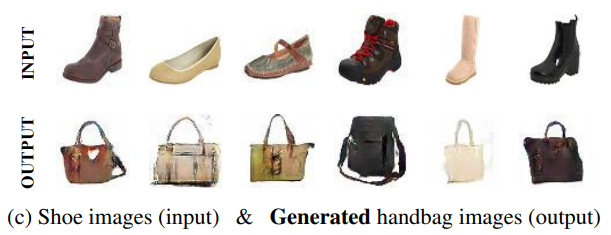
In the translation results shown in Figure 1, our proposed model discovers fashion style as a related feature between the two domains.
번역 된 결과는 유사한 색상과 패턴을 가질뿐만 아니라 입력 된 패션 아이템과 유사한 수준의 패션 형식을 가지고 있습니다.
Note that translated results not only have similar colors and patterns, but they also have similar level of fashion formality as the input fashion item.
번역 된 결과는 유사한 색상과 패턴을 가질뿐만 아니라 입력 된 패션 아이템과 유사한 수준의 패션 형식을 가지고 있습니다.
4. Related Work
Recently, a novel method to train generative models named Generative Adversarial Networks (GANs) (Goodfellow et al., 2014) was developed.
최근 GAN (Generative Adversarial Networks) (Goodfellow et al., 2014)이라는 생성 모델을 훈련하는 새로운 방법이 개발되었습니다.
A GAN is composed of two modules – a generator G and a discriminator D.
GAN은 생성기 G와 판별 기 D라는 두 개의 모듈로 구성됩니다.
The generator’s objective is to generate (synthesize) data samples whose distribution closely matches that of real data samples while the discriminator’s objective is to distinguish real ones from generated samples.
생성기의 목표는 분포가 실제 데이터 샘플의 분포와 거의 일치하는 데이터 샘플을 생성 (합성)하는 반면 판별 자의 목표는 생성 된 샘플과 실제 데이터를 구별하는 것입니다.
The two models G and D, formulated as a two-player minimax game, are trained simultaneously.
2 인용 미니 맥스 게임으로 구성된 두 모델 G와 D는 동시에 훈련됩니다.
Researchers have studied GANs vigorously in two years: network models such as LAPGAN (Denton et al., 2015) and DCGAN (Radford et al., 2016) and improved training techniques (Salimans et al., 2016; Arjovsky et al., 2017).
연구원들은 LAPGAN (Denton et al., 2015) 및 DCGAN (Radford et al., 2016)과 같은 네트워크 모델과 개선 된 훈련 기술 (Salimans et al., 2016; Arjovsky et al., 2017) 등 2 년 동안 GAN을 활발하게 연구했습니다. ).
More recent GAN works are described in (Goodfellow, 2017).
더 최근의 GAN 작품은 (Goodfellow, 2017)에 설명되어 있습니다.
Several methods were developed to generate images based on GANs.
GAN을 기반으로 이미지를 생성하기 위해 여러 가지 방법이 개발되었습니다.
Conditional Generative Adversarial Nets (cGANs) (Mirza & Osindero, 2014) use MNIST digit class label as an additional information to both generator and discriminator and can generate digit images of the specified class.
cGAN (Conditional Generative Adversarial Nets) (Mirza & Osindero, 2014)은 MNIST 숫자 클래스 레이블을 생성기와 판별 자 모두에 대한 추가 정보로 사용하고 지정된 클래스의 숫자 이미지를 생성 할 수 있습니다.
Similarly, Dosovitskiy et al. (2015) showed that GAN can generate images of objects based on specified characteristic codes such as color and viewpoint.
마찬가지로 Dosovitskiy et al. (2015)는 GAN이 색상 및 시점과 같은 특정 특성 코드를 기반으로 물체의 이미지를 생성 할 수 있음을 보여주었습니다.
Other approaches used conditional features from a completely different domain for image generation.
다른 접근법은 이미지 생성을 위해 완전히 다른 도메인의 조건부 기능을 사용했습니다.
For example, Reed et al. (2016) used encoded text description of images as the conditional information to generating images that match the description.
예를 들어, Reed et al. (2016)은 이미지의 인코딩 된 텍스트 설명을 조건부 정보로 사용하여 설명과 일치하는 이미지를 생성했습니다.
Some researchers have attempted to use multiple GANs in prior works.
일부 연구자들은 이전 작업에서 여러 GAN을 사용하려고 시도했습니다.
(Liu & Tuzel, 2016) proposed to couple two GANs (coupled generative adversarial networks, CoGAN) in which two generators and two discriminators are coupled by weight-sharing to learn the joint distribution of images in two different domains without using pair-wise data.
(Liu & Tuzel, 2016) 두 개의 생성기와 두 개의 판별자가 가중치 공유에 의해 결합되어 쌍별 데이터를 사용하지 않고 두 개의 다른 도메인에서 이미지의 공동 분포를 학습하는 두 개의 GAN (결합 된 생성 적대 네트워크, CoGAN)을 결합하도록 제안했습니다.
In Stacked GANs (StackGAN) (Zhang et al., 2016), two GANs are arranged sequentially where the Stage-I GAN generates low resolution images given text description and the Stage-II GAN improves the generated image into high resolution images.
Stacked GAN (StackGAN) (Zhang et al., 2016)에서는 Stage-I GAN이 텍스트 설명에 따라 저해상도 이미지를 생성하고 Stage-II GAN이 생성 된 이미지를 고해상도 이미지로 개선하는 두 개의 GAN이 순차적으로 배열됩니다.
Similarly, Style and Structure GAN (S2-GAN) (Wang & Gupta, 2016) used two sequentially connected GANs where the Structure GAN first generates surface normal image and the Style GAN transforms it into natural indoor scene image.
마찬가지로 Style and Structure GAN (S2-GAN) (Wang & Gupta, 2016)은 Structure GAN이 먼저 표면 일반 이미지를 생성하고 Style GAN이이를 자연스러운 실내 장면 이미지로 변환하는 두 개의 순차적으로 연결된 GAN을 사용했습니다.
In order to control specific attributes of an image, T. Kulkarni & P. Kohli (2015) proposed a method to disentangle specific factors by explicitly controlling target code.
이미지의 특정 속성을 제어하기 위해 T. Kulkarni & P. Kohli (2015)는 타겟 코드를 명시 적으로 제어하여 특정 요소를 분리하는 방법을 제안했습니다.
Perarnau et al. (2016) tackled image generation problems conditioned on specific attribute vectors by training an attribute predictor along with latent encoder.
Perarnau et al. (2016)은 잠재 인코더와 함께 속성 예측자를 훈련하여 특정 속성 벡터에 조건이 지정된 이미지 생성 문제를 해결했습니다.
In addition to using conditional information such as class labels and text encodings, several works in the field of image-to-image translation used images of one domain to generate images in another domain.
클래스 레이블 및 텍스트 인코딩과 같은 조건부 정보를 사용하는 것 외에도 이미지 대 이미지 변환 분야의 여러 작업에서는 한 도메인의 이미지를 사용하여 다른 도메인의 이미지를 생성했습니다.
(Isola et al., 2016) translated black-and-white images to colored images by training on paired black-and-white and colored image data.
(Isola et al., 2016) 쌍을 이루는 흑백 및 컬러 이미지 데이터를 학습하여 흑백 이미지를 컬러 이미지로 변환했습니다.
Similarly, Taigman et al. (2016) translated face images to emojis by providing image features from pre-trained face recognition module as conditional input to a GAN.
마찬가지로 Taigman et al. (2016)은 사전 훈련 된 얼굴 인식 모듈의 이미지 기능을 GAN에 대한 조건부 입력으로 제공하여 얼굴 이미지를 이모티콘으로 변환했습니다.
Recently, Tong et al. (2017) tackled mode-collapsing and instability problems in GAN training.
최근 Tong et al. (2017) GAN 교육에서 모드 축소 및 불안정 문제를 해결했습니다
They introduced two ways of regularizing general GAN objective – geometric metrics regularizer and mode regularizer.
그들은 일반적인 GAN 목표를 정규화하는 두 가지 방법 인 기하학적 메트릭 정규화 기와 모드 정규화를 도입했습니다.
5. Conclusion
This paper presents a learning method to discover crossdomain relations with a generative adversarial network called DiscoGAN. Our approach works without any explicit pair labels and learns to relate datasets from very different domains.
이 논문은 DiscoGAN이라는 생성 적 적대 네트워크와 교차 도메인 관계를 발견하는 학습 방법을 제시합니다. 우리의 접근 방식은 명시적인 쌍 레이블없이 작동하며 매우 다른 도메인의 데이터 세트를 연결하는 방법을 배웁니다.
We have demonstrated that DiscoGAN can generate high-quality images with transferred style.
DiscoGAN이 전송 된 스타일로 고품질 이미지를 생성 할 수 있음을 입증했습니다.
One possible future direction is to modify DiscoGAN to handle mixed modalities (e.g. text and image).
한 가지 가능한 미래 방향은 혼합 양식 (예 : 텍스트 및 이미지)을 처리하도록 DiscoGAN을 수정하는 것입니다
'비지도학습 > GAN' 카테고리의 다른 글
| [2주차] GAN (수정중) (0) | 2021.01.28 |
|---|---|
| [1주차] AE/VAE/GAN(수정중) (0) | 2021.01.28 |
| [7주차] Unpaired Image-to-Image Translation using Cycle-Consistent Adversarial Networks, 2020 (0) | 2021.01.28 |
| [6주차] Image-to-Image Translation with Conditional Adversarial Networks, 2018 (0) | 2021.01.28 |
| [5주차]Conditional Generative Adversarial Network, 2014 (0) | 2021.01.27 |


