PROGRESSIVE GROWING OF GANS FOR IMPROVED QUALITY, STABILITY, AND VARIATION(NVIDIA,2019)
ABSTRACT
We describe a new training methodology for generative adversarial networks.
The key idea is to grow both the generator and discriminator progressively: starting from a low resolution, we add new layers that model increasingly fine details as training progresses.
This both speeds the training up and greatly stabilizes it, allowing us to produce images of unprecedented quality, e.g., CELEBA images at 10242 .
We also propose a simple way to increase the variation in generated images, and achieve a record inception score of 8.80 in unsupervised CIFAR10.
Additionally, we describe several implementation details that are important for discouraging unhealthy competition between the generator and discriminator.
Finally, we suggest a new metric for evaluating GAN results, both in terms of image quality and variation.
As an additional contribution, we construct a higher-quality version of the CELEBA dataset.
생성적 적대 네트워크에 대한 새로운 훈련 방법론을 설명합니다.
핵심 아이디어는 생성기와 판별기를 점진적으로 성장시키는 것입니다.
저해상도부터 시작하여 훈련이 진행됨에 따라 점점 더 미세한 세부 사항을 모델링하는 새로운 레이어를 추가합니다.
이를 통해 훈련 속도를 높이고, 이를 크게 안정화시켜 전례없는 품질의 이미지를 생성 할 수 있습니다 (예 : 10242의 CELEBA 이미지).
또한 생성된 이미지의 변화를 늘리고 감독되지 않은 CIFAR10에서 8.80의 기록 시작 점수를 달성하는 간단한 방법을 제안합니다.
또한 생성자와 판별 자 간의 불건전 한 경쟁을 막는 데 중요한 몇 가지 구현 세부 정보를 설명합니다.
마지막으로, 이미지 품질 및 변형 측면에서 GAN 결과를 평가하기위한 새로운 메트릭을 제안합니다.
추가 기여로 CELEBA 데이터 세트의 고품질 버전을 구성합니다.
1 INTRODUCTION
Generative methods that produce novel samples from high-dimensional data distributions, such as images, are finding widespread use, for example in speech synthesis (van den Oord et al., 2016a), image-to-image translation (Zhu et al., 2017; Liu et al., 2017; Wang et al., 2017), and image inpainting (Iizuka et al., 2017).
Currently the most prominent approaches are autoregressive models (van den Oord et al., 2016b;c), variational autoencoders (VAE) (Kingma & Welling, 2014), and generative adversarial networks (GAN) (Goodfellow et al., 2014). Currently they all have significant strengths and weaknesses.
Autoregressive models – such as PixelCNN – produce sharp images but are slow to evaluate and do not have a latent representation as they directly model the conditional distribution over pixels, potentially limiting their applicability.
VAEs are easy to train but tend to produce blurry results due to restrictions in the model, although recent work is improving this (Kingma et al., 2016). GANs produce sharp images, albeit only in fairly small resolutions and with somewhat limited variation, and the training continues to be unstable despite recent progress (Salimans et al., 2016; Gulrajani et al., 2017; Berthelot et al., 2017; Kodali et al., 2017).
Hybrid methods combine various strengths of the three, but so far lag behind GANs in image quality (Makhzani & Frey, 2017; Ulyanov et al., 2017; Dumoulin et al., 2016).
이미지와 같은 고차원 데이터 분포에서 새로운 샘플을 생성하는 생성 방법은 예를 들어 음성 합성 (van den Oord et al., 2016a), 이미지 대 이미지 번역 (Zhu et al., 2017; Liu et al., 2017; Wang et al., 2017) 및 이미지 인 페인팅 (Iizuka et al., 2017). 현재 가장 눈에 띄는 접근 방식은 자기 회귀 모델 autoregressive (van den Oord et al., 2016b; c), VAE (variational autoencoder) (Kingma & Welling, 2014) 및 생성적 적대 네트워크 (GAN) (Goodfellow et al., 2014)입니다.
현재 그들은 모두 상당한 강점과 약점을 가지고 있습니다.
PixelCNN과 같은 자기 회귀 모델은 선명한 이미지를 생성하지만 평가 속도가 느리고 픽셀에 대한 조건부 분포를 직접 모델링하므로 잠재적으로 적용 가능성을 제한하기 때문에 잠재 표현이 없습니다.
VAE는 학습하기 쉽지만 최근 작업이 이를 개선하고 있지만 모델의 제한으로 인해 흐릿한 결과를 생성하는 경향이 있습니다 (Kingma et al., 2016).
GAN은 매우 작은 해상도와 다소 제한적인 변형으로 만 선명한 이미지를 생성하며 최근의 진행에도 불구하고 훈련이 계속 불안정합니다 (Salimans et al., 2016; Gulrajani et al., 2017; Berthelot et al., 2017; Kodali et al., 2017).
하이브리드 방법은 세 가지의 다양한 강점을 결합하지만 이미지 품질면에서 GAN보다 훨씬 뒤떨어져 있습니다 (Makhzani & Frey, 2017; Ulyanov et al., 2017; Dumoulin et al., 2016).
Typically, a GAN consists of two networks: generator and discriminator (aka critic).
The generator produces a sample, e.g., an image, from a latent code, and the distribution of these images should ideally be indistinguishable from the training distribution.
Since it is generally infeasible to engineer a function that tells whether that is the case, a discriminator network is trained to do the assessment, and since networks are differentiable, we also get a gradient we can use to steer both networks to the right direction.
Typically, the generator is of main interest – the discriminator is an adaptive loss function that gets discarded once the generator has been trained.
일반적으로 GAN은 생성기와 판별자 (일명 비평가)의 두 네트워크로 구성됩니다.
생성기는 잠재 코드에서 이미지 (예 : 이미지)를 생성하며 이러한 이미지의 분포는 훈련 분포와 이상적으로 구별 할 수 없습니다.
그런 경우인지 여부를 알려주는 함수를 설계하는 것은 일반적으로 불가능하기 때문에 판별기 네트워크는 평가를 수행하도록 훈련되고 네트워크는 미분 가능하므로 두 네트워크를 올바른 방향으로 조정하는 데 사용할 수있는 기울기도 얻습니다.
일반적으로 생성기는 주요 관심사입니다.
판별기는 생성기가 훈련되면 폐기되는 적응형 손실 함수(adaptive loss function)입니다.
There are multiple potential problems with this formulation.
When we measure the distance between the training distribution and the generated distribution, the gradients can point to more or less random directions if the distributions do not have substantial overlap, i.e., are too easy to tell apart (Arjovsky & Bottou, 2017).
Originally, Jensen-Shannon divergence was used as a distance metric (Goodfellow et al., 2014), and recently that formulation has been improved (Hjelm et al., 2017) and a number of more stable alternatives have been proposed, including least squares (Mao et al., 2016b), absolute deviation with margin (Zhao et al., 2017), and Wasserstein distance (Arjovsky et al., 2017; Gulrajaniet al., 2017).
Our contributions are largely orthogonal to this ongoing discussion, and we primarily use the improved Wasserstein loss, but also experiment with least-squares loss.
이 공식에는 여러 가지 잠재적인 문제가 있습니다.
훈련 분포와 생성된 분포 사이의 거리를 측정할 때 분포가 상당히 겹치지 않는 경우, 즉 구분하기가 너무 쉬운 경우 기울기는 다소 랜덤한 방향을 가리킬 수 있습니다 (Arjovsky & Bottou, 2017).
원래 Jensen-Shannon 발산은 거리 측정법으로 사용되었으며 (Goodfellow et al., 2014) 최근에는 그 공식이 개선되었으며, (Hjelm et al., 2017) 최소 제곱(Mao et al., 2016b), 여백에 따른 절대 편차 (Zhao et al., 2017), Wasserstein 거리 (Arjovsky et al., 2017; Gulrajaniet al., 2017)을 포함하여 더 안정된 대안이 제안되었습니다.
우리의 기여는이 진행중인 논의에 대체로 직교(orthogonal)하며 개선된 Wasserstein 손실을 주로 사용하지만 최소 제곱 손실도 실험합니다.
The generation of high-resolution images is difficult because higher resolution makes it easier to tell the generated images apart from training images (Odena et al., 2017), thus drastically amplifying the gradient problem.
Large resolutions also necessitate using smaller minibatches due to memory constraints, further compromising training stability.
Our key insight is that we can grow both the generator and discriminator progressively, starting from easier low-resolution images, and add new layers that introduce higher-resolution details as the training progresses.
This greatly speeds up training and improves stability in high resolutions, as we will discuss in Section 2.
고해상도 이미지의 생성은 더 높은 해상도는 생성된 이미지를 훈련 이미지와 구별하기 쉽게하여 (Odena et al., 2017) 그래디언트 문제를 크게 증폭시키기 때문에 어렵습니다.
해상도가 크면 메모리 제약으로 인해 더 작은 미니 배치를 사용해야하므로 훈련 안정성이 더욱 저하됩니다.
우리의 핵심 통찰력은 더 쉬운 저해상도 이미지에서 시작하여 생성기와 판별기를 점진적으로 성장시키고 훈련이 진행됨에 따라 고해상도 세부 사항을 도입하는 새로운 레이어를 추가 할 수 있다는 것입니다.
이는 섹션 2에서 논의 할 것이므로 높은 해상도에서 훈련 속도를 크게 높이고 안정성을 향상시킵니다.
The GAN formulation does not explicitly require the entire training data distribution to be represented by the resulting generative model.
The conventional wisdom has been that there is a tradeoff between image quality and variation, but that view has been recently challenged (Odena et al., 2017). The degree of preserved variation is currently receiving attention and various methods have been suggested for measuring it, including inception score (Salimans et al., 2016), multi-scale structural similarity (MS-SSIM) (Odena et al., 2017; Wang et al., 2003), birthday paradox (Arora & Zhang, 2017), and explicit tests for the number of discrete modes discovered (Metz et al., 2016). We will describe our method for encouraging variation in Section 3, and propose a new metric for evaluating the quality and variation in Section 5.
GAN 공식은 전체 학습 데이터 분포가 결과 생성 모델로 표현되도록 명시적으로 요구하지 않습니다.
이미지 품질과 변형 사이에는 상충 관계(tradeoff)가 있다는 것이 일반적인 통념이지만 최근에는 그 관점에 도전이되었습니다 (Odena et al., 2017).
보존된 변이(preserved variation)의 정도는 현재 주목을 받고 있으며, 개시 점수 inception score (Salimans et al., 2016), 다중 스케일 구조 유사성 multi-scale structural similarity(MS-SSIM) (Odena et al., 2017; Wang et al., 2003), 생일 패러독스birthday paradox (Arora & Zhang, 2017), 발견 된 이산 모드의 수에 대한 명시적 테스트explicit tests for the number of discrete modes discovered (Metz et al., 2016).
섹션 3에서 변동을 장려하는 방법을 설명하고 섹션 5에서 품질 및 변동을 평가하기위한 새로운 메트릭을 제안합니다.
Section 4.1 discusses a subtle modification to the initialization of networks, leading to a more balanced learning speed for different layers.
Furthermore, we observe that mode collapses traditionally plaguing GANs tend to happen very quickly, over the course of a dozen minibatches.
Commonly they start when the discriminator overshoots, leading to exaggerated gradients, and an unhealthy competition follows where the signal magnitudes escalate in both networks.
We propose a mechanism to stop the generator from participating in such escalation, overcoming the issue (Section 4.2).
섹션 4.1에서는 네트워크 초기화에 대한 미묘한 수정을 논의하여 다른 계층에 대해보다 균형 잡힌 학습 속도를 제공합니다.
또한, 모드 붕괴는 전통적으로 GAN을 괴롭히는 GAN이 수십 개의 미니 배치 과정에서 매우 빠르게 발생하는 경향이 있음을 관찰합니다.
일반적으로 판별기가 오버슈팅하여 과장된 기울기로 이어질 때 시작되며 두 네트워크에서 신호 크기가 증가하는 비정상적인 경쟁이 뒤따릅니다.
생성자가 이러한 에스컬레이션에 참여하지 못하도록하여 문제를 극복하는 메커니즘을 제안합니다 (섹션 4.2).
We evaluate our contributions using the CELEBA, LSUN, CIFAR10 datasets.
We improve the best published inception score for CIFAR10.
Since the datasets commonly used in benchmarking generative methods are limited to a fairly low resolution, we have also created a higher quality version of the CELEBA dataset that allows experimentation with output resolutions up to 1024 × 1024 pixels.
This dataset and our full implementation are available at https://github.com/tkarras/progressive_growing_of_gans, trained networks can be found at https://drive.google.com/open?id=0B4qLcYyJmiz0NHFULTdYc05lX0U along with result images, and a supplementary video illustrating the datasets, additional results, and latent space interpolations is at https://youtu.be/G06dEcZ-QTg.
CELEBA, LSUN, CIFAR10 데이터 세트를 사용하여 우리의 기여를 평가합니다.
CIFAR10에 대해 가장 잘 게시 된 시작 점수를 개선합니다.
생성 방법을 벤치마킹하는데 일반적으로 사용되는 데이터 세트는 상당히 낮은 해상도로 제한되기 때문에 최대 1024 × 1024 픽셀의 출력 해상도로 실험 할 수있는 CELEBA 데이터 세트의 고품질 버전도 만들었습니다.
이 데이터 세트와 전체 구현은 https://github.com/tkarras/progressive_growing_of_gans에서 사용할 수 있으며 학습된 네트워크는 https://drive.google.com/open?id=0B4qLcYyJmiz0NHFULTdYc05lX0U에서 결과 이미지와 함께 찾을 수 있습니다.
데이터 세트, 추가 결과 및 잠재 공간 보간을 보여주는 비디오는 https://youtu.be/G06dEcZ-QTg에 있습니다.
2 PROGRESSIVE GROWING OF GANS


Our primary contribution is a training methodology for GANs where we start with low-resolution images, and then progressively increase the resolution by adding layers to the networks as visualized in Figure 1.
This incremental nature allows the training to first discover large-scale structure of the image distribution and then shift attention to increasingly finer scale detail, instead of having to learn all scales simultaneously.
우리의 주요 기여는 저해상도 이미지로 시작한 다음 그림 1에서 시각화 된 것처럼 네트워크에 계층을 추가하여 해상도를 점진적으로 높이는 GAN을위한 교육 방법론입니다.
이러한 점진적 특성 덕분에 교육은 먼저 이미지 분포의 대규모 구조를 발견 한 다음 모든 스케일을 동시에 학습 할 필요없이 점점 더 미세한 스케일 세부 사항으로주의를 전환 할 수 있습니다.
We use generator and discriminator networks that are mirror images of each other and always grow in synchrony.
All existing layers in both networks remain trainable throughout the training process.
When new layers are added to the networks, we fade them in smoothly, as illustrated in Figure 2.
This avoids sudden shocks to the already well-trained, smaller-resolution layers.
Appendix A describes structure of the generator and discriminator in detail, along with other training parameters.
우리는 서로의 거울 이미지이며 항상 동기화되어 성장하는 생성기 및 판별기 네트워크를 사용합니다.
두 네트워크의 모든 기존 계층은 훈련 과정 내내 훈련 가능한 상태로 유지됩니다.
새 레이어가 네트워크에 추가되면 그림 2와 같이 부드럽게 페이드 인 됩니다.
이렇게하면 이미 잘 훈련된 더 작은 해상도 레이어에 대한 갑작스런 충격을 방지 할 수 있습니다.
부록 A는 다른 훈련 매개 변수와 함께 생성기 및 판별기의 구조를 자세히 설명합니다.
We observe that the progressive training has several benefits. Early on, the generation of smaller images is substantially more stable because there is less class information and fewer modes (Odena et al., 2017).
By increasing the resolution little by little we are continuously asking a much simpler question compared to the end goal of discovering a mapping from latent vectors to e.g. 10242 images.
This approach has conceptual similarity to recent work by Chen & Koltun (2017). In practice it stabilizes the training sufficiently for us to reliably synthesize megapixel-scale images using WGAN-GP loss (Gulrajani et al., 2017) and even LSGAN loss (Mao et al., 2016b).
우리는 점진적 훈련이 몇 가지 이점이 있음을 관찰합니다.
초기에 더 작은 이미지의 생성은 클래스 정보가 적고 모드가 적기 때문에 훨씬 더 안정적입니다 (Odena et al., 2017).
해상도를 조금씩 늘림으로써 우리는 잠재 벡터에서 예를 들어 매핑을 발견하는 최종 목표에 비해 훨씬 더 간단한 질문을 계속하고 있습니다.
10242 이미지. 이 접근 방식은 Chen & Koltun (2017)의 최근 작업과 개념적으로 유사합니다.
실제로 WGAN-GP 손실 (Gulrajani et al., 2017) 및 LSGAN 손실 (Mao et al., 2016b)을 사용하여 메가 픽셀 스케일 이미지를 안정적으로 합성할 수 있도록 훈련을 충분히 안정화합니다.
Another benefit is the reduced training time. With progressively growing GANs most of the iterations are done at lower resolutions, and comparable result quality is often obtained up to 2–6 times faster, depending on the final output resolution.
The idea of growing GANs progressively is related to the work of Wang et al. (2017), who use multiple discriminators that operate on different spatial resolutions.
또 다른 이점은 학습 시간 단축입니다.
점진적으로 증가하는 GAN으로 대부분의 반복은 더 낮은 해상도에서 수행되며 최종 출력 해상도에 따라 비슷한 결과 품질을 최대 2 ~ 6 배 더 빠르게 얻을 수 있습니다.
점진적으로 GAN을 성장시키는 아이디어는 Wang et al. (2017), 다른 공간 해상도에서 작동하는 다중 판별자를 사용합니다.
That work in turn is motivated by Durugkar et al. (2016) who use one generator and multiple discriminators concurrently, and Ghosh et al. (2017) who do the opposite with multiple generators and one discriminator.
Hierarchical GANs (Denton et al., 2015; Huang et al., 2016; Zhang et al., 2017) define a generator and discriminator for each level of an image pyramid.
These methods build on the same observation as our work – that the complex mapping from latents to high-resolution images is easier to learn in steps – but the crucial difference is that we have only a single GAN instead of a hierarchy of them.
In contrast to early work on adaptively growing networks, e.g., growing neural gas (Fritzke, 1995) and neuro evolution of augmenting topologies (Stanley & Miikkulainen, 2002) that grow networks greedily, we simply defer the introduction of pre-configured layers.
In that sense our approach resembles layer-wise training of autoencoders (Bengio et al., 2007).
그 작업은 Durugkar et al. (2016)은 하나의 생성기와 여러 개의 판별자를 동시에 사용하고 Ghosh et al. (2017) 누가 여러 생성기와 하나의 판별 자로 반대를 수행합니다.
계층적 GAN (Denton et al., 2015; Huang et al., 2016; Zhang et al., 2017)은 이미지 피라미드의 각 수준에 대한 생성기와 판별자를 정의합니다.
이러한 방법은 잠복에서 고해상도 이미지로의 복잡한 매핑이 단계적으로 학습하기 더 쉽다는 우리 작업과 동일한 관찰을 기반으로하지만 결정적인 차이점은 계층 구조 대신 단일 GAN 만 있다는 것입니다.
적응적으로 성장하는 네트워크에 대한 초기 연구, 예를 들어 성장하는 신경 가스 (Fritzke, 1995) 및 네트워크를 탐욕스럽게 성장시키는 증강 토폴로지의 신경 진화 (Stanley & Miikkulainen, 2002)와는 달리, 우리는 단순히 미리 구성된 레이어의 도입을 연기합니다.
그런 의미에서 우리의 접근 방식은 오토 인코더의 계층별 교육과 유사합니다 (Bengio et al., 2007).
3 INCREASING VARIATION USING MINIBATCH STANDARD DEVIATION 미니 배치 표준 편차를 사용하여 변동 증가
GANs have a tendency to capture only a subset of the variation found in training data, and Salimans et al. (2016) suggest “minibatch discrimination” as a solution.
They compute feature statistics not only from individual images but also across the minibatch, thus encouraging the minibatches of generated and training images to show similar statistics.
This is implemented by adding a minibatch layer towards the end of the discriminator, where the layer learns a large tensor that projects the input activation to an array of statistics.
A separate set of statistics is produced for each example in a minibatch and it is concatenated to the layer’s output, so that the discriminator can use the statistics internally.
We simplify this approach drastically while also improving the variation.
GAN은 훈련 데이터에서 발견 된 변동의 하위 집합만 캡처하는 경향이 있으며 Salimans et al. (2016)은 해결책으로“미니 배치 판별”을 제안했습니다.
개별 이미지뿐만 아니라 미니 배치 전체에서 특징 통계를 계산하므로 생성 된 이미지와 훈련 이미지의 미니 배치가 유사한 통계를 표시하도록 장려합니다. 이것은 식별기의 끝에 미니 배치 계층을 추가하여 구현됩니다.
여기서 계층은 입력 활성화를 통계 배열에 투영하는 큰 텐서를 학습합니다.
미니 배치의 각 예제에 대해 별도의 통계 세트가 생성되고 계층의 출력에 연결되어 판별자가 통계를 내부적으로 사용할 수 있습니다.
이 접근 방식을 대폭 단순화하는 동시에 변형도 개선합니다.
Our simplified solution has neither learnable parameters nor new hyperparameters.
We first compute the standard deviation for each feature in each spatial location over the minibatch. We then average these estimates over all features and spatial locations to arrive at a single value. We replicate the value and concatenate it to all spatial locations and over the minibatch, yielding one additional (constant) feature map.
This layer could be inserted anywhere in the discriminator, but we have found it best to insert it towards the end (see Appendix A.1 for details).
We experimented with a richer set of statistics, but were not able to improve the variation further. In parallel work, Lin et al. (2017) provide theoretical insights about the benefits of showing multiple images to the discriminator.
Alternative solutions to the variation problem include unrolling the discriminator (Metz et al., 2016) to regularize its updates, and a “repelling regularizer” (Zhao et al., 2017) that adds a new loss term to the generator, trying to encourage it to orthogonalize the feature vectors in a minibatch.
The multiple generators of Ghosh et al. (2017) also serve a similar goal. We acknowledge that these solutions may increase the variation even more than our solution – or possibly be orthogonal to it – but leave a detailed comparison to a later time.
단순화된 솔루션에는 학습 가능한 매개변수나 새로운 하이퍼파라미터가 없습니다.
먼저 미니 배치를 통해 각 공간 위치의 각 기능에 대한 표준 편차를 계산합니다.
그런 다음 모든 기능 및 공간 위치에 대해 이러한 추정치를 평균하여 단일 값에 도달합니다.
값을 복제하고 모든 공간 위치와 미니 배치에 연결하여 하나의 추가 (상수) feature map을 생성합니다.
이 레이어는 판별기의 아무 곳에 나 삽입 할 수 있지만 끝쪽으로 삽입하는 것이 가장 좋습니다 (자세한 내용은 부록 A.1 참조).
더 풍부한 통계 세트로 실험했지만 유사 콘텐츠를 더 개선 할 수 없었습니다.
병렬 작업에서 Lin et al. (2017)은 판별자에게 여러 이미지를 표시 할 때의 이점에 대한 이론적 통찰력을 제공합니다.
변형 문제에 대한 대체 솔루션에는 식별기 (Metz et al., 2016)를 풀고 업데이트를 정규화하는 것과 생성기에 새로운 손실 항을 추가하는 “반복 정규화”(Zhao et al., 2017)가 있습니다.
미니 배치에서 특징 벡터를 직교화합니다.
Ghosh et al.의 여러 생성기. (2017)도 비슷한 목표를 달성합니다.
우리는 이러한 솔루션이 우리의 솔루션보다 훨씬 더 변동을 증가시킬 수 있음을 인정하지만 (또는 그것에 직교 할 수 있음) 나중에 자세한 비교를 남겨 둡니다.
4 NORMALIZATION IN GENERATOR AND DISCRIMINATOR 생성자 및 차별자의 정규화
GANs are prone to the escalation of signal magnitudes as a result of unhealthy competition between the two networks.
Most if not all earlier solutions discourage this by using a variant of batch normalization (Ioffe & Szegedy, 2015; Salimans & Kingma, 2016; Ba et al., 2016) in the generator, and often also in the discriminator.
These normalization methods were originally introduced to eliminate covariate shift.
However, we have not observed that to be an issue in GANs, and thus believe that the actual need in GANs is constraining signal magnitudes and competition.
We use a different approach that consists of two ingredients, neither of which include learnable parameters.
GAN은 두 네트워크 간의 비정상적인 경쟁으로 인해 신호 크기가 증가하는 경향이 있습니다.
대부분의 초기 솔루션은 생성기 및 종종 판별기에서 배치 정규화 변형 (Ioffe & Szegedy, 2015; Salimans & Kingma, 2016; Ba et al., 2016)을 사용하여이를 방지합니다.
이러한 정규화 방법은 원래 공변량 이동(covariate shift)을 제거하기 위해 도입되었습니다.
그러나 우리는 GAN에서 문제가되는 것을 관찰하지 않았으므로 GAN의 실제 요구가 신호 크기와 경쟁을 제한하고 있다고 믿습니다.
학습 가능한 매개 변수를 포함하지 않는 두 가지 요소로 구성된 다른 접근 방식을 사용합니다.
4.1 EQUALIZED LEARNING RATE 동등한 학습률
We deviate from the current trend of careful weight initialization, and instead use a trivial N (0, 1) initialization and then explicitly scale the weights at runtime. To be precise, we set wˆi = wi/c, where wi are the weights and c is the per-layer normalization constant from He’s initializer (He et al., 2015).
The benefit of doing this dynamically instead of during initialization is somewhat subtle, and relates to the scale-invariance in commonly used adaptive stochastic gradient descent methods such as RMSProp (Tieleman & Hinton, 2012) and Adam (Kingma & Ba, 2015).
These methods normalize a gradient update by its estimated standard deviation, thus making the update independent of the scale of the parameter.
As a result, if some parameters have a larger dynamic range than others, they will take longer to adjust.
This is a scenario modern initializers cause, and thus it is possible that a learning rate is both too large and too small at the same time.
Our approach ensures that the dynamic range, and thus the learning speed, is the same for all weights.
A similar reasoning was independently used by van Laarhoven (2017).
신중한 가중치 초기화의 현재 추세에서 벗어나 대신 간단한 N (0, 1) 초기화를 사용한 다음 런타임에 가중치를 명시적으로 조정합니다.
정확히 말하면 $wˆi= w_i/c$로 설정합니다.
여기서 $w_i$는 가중치이고 $c$는 $He$의 이니셜 라이저의 레이어 별 정규화 상수입니다 (He et al., 2015).
초기화하는 동안 대신 동적으로 수행하는 이점은 다소 미묘하며 RMSProp (Tieleman & Hinton, 2012) 및 Adam (Kingma & Ba, 2015)과 같이 일반적으로 사용되는 적응형 확률적 경사하강 법의 척도 불변과 관련이 있습니다.
이러한 방법은 추정된 표준 편차로 기울기 업데이트를 정규화하므로 매개 변수의 척도와 독립적으로 업데이트됨
결과적으로 일부 매개 변수의 동적 범위가 다른 매개 변수보다 큰 경우 조정하는 데 시간이 더 오래 걸립니다.
이것은 현대 이니셜라이저가 야기하는 시나리오이므로 학습률이 동시에 너무 크고 너무 작을 수 있습니다.
우리의 접근 방식은 동적 범위, 즉 학습 속도가 모든 가중치에 대해 동일하다는 것을 보장합니다.
유사한 추론이 van Laarhoven (2017)에 의해 독립적으로 사용되었습니다.
4.2 PIXELWISE FEATURE VECTOR NORMALIZATION IN GENERATOR 생성기의 픽셀 단위 기능 벡터 정규화
To disallow the scenario where the magnitudes in the generator and discriminator spiral out of control as a result of competition, we normalize the feature vector in each pixel to unit length in the generator after each convolutional layer. We do this using a variant of “local response normalization” (Krizhevsky et al., 2012), configured as bx,y = ax,y/ q 1 N PN−1 j=0 (a j x,y) 2 + , where = 10−8 , N is the number of feature maps, and ax,y and bx,y are the original and normalized feature vector in pixel (x, y), respectively.
We find it surprising that this heavy-handed constraint does not seem to harm the generator in any way, and indeed with most datasets it does not change the results much, but it prevents the escalation of signal magnitudes very effectively when needed.
경쟁의 결과로 발생기 및 판별기의 크기가 제어 범위를 벗어난 시나리오를 허용하지 않기 위해 각 컨벌루션 계층 이후의 생성기에서 각 픽셀의 특징 벡터를 생성기의 단위 길이로 정규화합니다.
우리는 $bx,y=ax,y/q1NPN-1j=0(ajx,y)2+$ $=10-8,$로 구성된 "로컬 응답 정규화"(Krizhevsky et al., 2012)의 변형을 사용하여이를 수행합니다.
N은 특징 맵의 수이고 ax, y 및 bx, y는 각각 픽셀 (x, y)의 원래 및 정규화 된 특징 벡터입니다.
이 과중한 제약이 어떤 식으로든 생성기에 해를 끼치지 않는 것 같고 실제로 대부분의 데이터 세트에서 결과를 많이 변경하지는 않지만 필요할 때 신호 크기의 에스컬레이션을 매우 효과적으로 방지한다는 것이 놀랍습니다.
5 MULTI-SCALE STATISTICAL SIMILARITY FOR ASSESSING GAN RESULTS
In order to compare the results of one GAN to another, one needs to investigate a large number of images, which can be tedious, difficult, and subjective.
Thus, it is desirable to rely on automated methods that compute some indicative metric from large image collections.
We noticed that existing methods such as MS-SSIM (Odena et al., 2017) find large-scale mode collapses reliably but fail to react to smaller effects such as loss of variation in colors or textures, and they also do not directly assess image quality in terms of similarity to the training set.
We build on the intuition that a successful generator will produce samples whose local image structure is similar to the training set over all scales.
We propose to study this by considering the multiscale statistical similarity between distributions of local image patches drawn from Laplacian pyramid (Burt & Adelson, 1987) representations of generated and target images, starting at a low-pass resolution of 16 × 16 pixels.
As per standard practice, the pyramid progressively doubles until the full resolution is reached, each successive level encoding the difference to an up-sampled version of the previous level.
한 GAN의 결과를 다른 GAN과 비교하려면 지루하고 어렵고 주관적일 수있는 많은 수의 이미지를 조사해야합니다.
따라서 대규모 이미지 컬렉션에서 일부 지표를 계산하는 자동화 된 방법에 의존하는 것이 바람직합니다.
MS-SSIM (Odena et al., 2017)과 같은 기존 방법은 대규모 모드가 안정적으로 붕괴되지만 색상 또는 질감의 변화와 같은 작은 효과에는 반응하지 않으며 이미지를 직접 평가하지 않습니다.
훈련 세트와의 유사성 측면에서 품질. 우리는 성공적인 제너레이터가 로컬 이미지 구조가 모든 척도에서 훈련 세트와 유사한 샘플을 생성 할 것이라는 직관을 기반으로합니다.
우리는 16 × 16 픽셀의 저역 통과 해상도에서 시작하여 생성 된 이미지와 대상 이미지의 Laplacian 피라미드 (Burt & Adelson, 1987) 표현에서 가져온 로컬 이미지 패치 분포 간의 다중 스케일 통계적 유사성을 고려하여이를 연구 할 것을 제안합니다.
표준 관행에 따라 피라미드는 전체 해상도에 도달 할 때까지 점진적으로 두 배가되며 각 연속 레벨은 이전 레벨의 업 샘플링 된 버전으로 차이를 인코딩합니다.
A single Laplacian pyramid level corresponds to a specific spatial frequency band.
We randomly sample 16384 images and extract 128 descriptors from each level in the Laplacian pyramid, giving us 2 21 (2.1M) descriptors per level. Each descriptor is a 7 × 7 pixel neighborhood with 3 color channels, denoted by x ∈ R 7×7×3 = R 147.
We denote the patches from level l of the training set and generated set as {x l i } 2 21 i=1 and {y l i } 2 21 i=1, respectively.
We first normalize {x l i } and {y l i } w.r.t. the mean and standard deviation of each color channel, and then estimate the statistical similarity by computing their sliced Wasserstein distance SWD({x l i }, {y l i }), an efficiently computable randomized approximation to earthmovers distance, using 512 projections (Rabin et al., 2011).
단일 라플라시안 피라미드 레벨은 특정 공간 주파수 대역에 해당합니다. 우리는 무작위로 16384 개의 이미지를 샘플링하고 라플라시안 피라미드의 각 레벨에서 128 개의 설명자를 추출하여 레벨 당 2 개의 21 (2.1M) 설명자를 제공합니다. 각 설명자는 x ∈ R 7x7x3 = R 147로 표시되는 3 개의 색상 채널이있는 7 x 7 픽셀 이웃입니다. 훈련 세트 레벨 l의 패치와 생성 된 세트를 각각 {x l i} 2 21 i = 1 및 {y l i} 2 21 i = 1로 표시합니다. 먼저 {x l i} 및 {y l i} w.r.t를 정규화합니다. 각 색상 채널의 평균 및 표준 편차를 계산 한 다음 512 개의 투영을 사용하여 효율적으로 계산할 수있는 earthmovers 거리에 대한 무작위 근사값 인 슬라이스 Wasserstein 거리 SWD ({xli}, {yli})를 계산하여 통계적 유사성을 추정합니다 (Rabin et al. , 2011).
Intuitively a small Wasserstein distance indicates that the distribution of the patches is similar, meaning that the training images and generator samples appear similar in both appearance and variation at this spatial resolution.
In particular, the distance between the patch sets extracted from the lowestresolution 16 × 16 images indicate similarity in large-scale image structures, while the finest-level patches encode information about pixel-level attributes such as sharpness of edges and noise.
직관적으로, 작은 Wasserstein 거리는 패치의 분포가 유사하다는 것을 나타냅니다. 즉, 훈련 이미지와 생성기 샘플이이 공간 해상도에서 모양과 변동이 비슷하게 나타납니다. 특히, 가장 낮은 해상도의 16x16 이미지에서 추출 된 패치 세트 간의 거리는 대규모 이미지 구조에서 유사성을 나타내는 반면, 최고 수준의 패치는 가장자리의 선명도 및 노이즈와 같은 픽셀 수준 속성에 대한 정보를 인코딩합니다.
6 EXPERIMENTS
In this section we discuss a set of experiments that we conducted to evaluate the quality of our results. Please refer to Appendix A for detailed description of our network structures and training configurations.
We also invite the reader to consult the accompanying video (https://youtu.be/G06dEcZ-QTg) for additional result images and latent space interpolations. In this section we will distinguish between the network structure (e.g., convolutional layers, resizing), training configuration (various normalization layers, minibatch-related operations), and training loss (WGAN-GP, LSGAN).
이 섹션에서는 결과의 품질을 평가하기 위해 수행 한 일련의 실험에 대해 설명합니다.
네트워크 구조 및 교육 구성에 대한 자세한 설명은 부록 A를 참조하십시오.
또한 추가 결과 이미지 및 잠재 공간 보간을 위해 독자가 첨부 된 비디오 (https://youtu.be/G06dEcZ-QTg)를 참조하도록 초대합니다.
이 섹션에서는 네트워크 구조 (예 : 컨볼 루션 계층, 크기 조정), 훈련 구성 (다양한 정규화 계층, 미니 배치 관련 작업) 및 훈련 손실 (WGAN-GP, LSGAN)을 구분합니다.
6.1 IMPORTANCE OF INDIVIDUAL CONTRIBUTIONS IN TERMS OF STATISTICAL SIMILARITY
We will first use the sliced Wasserstein distance (SWD) and multi-scale structural similarity (MSSSIM) (Odena et al., 2017) to evaluate the importance our individual contributions, and also perceptually validate the metrics themselves.
We will do this by building on top of a previous state-of-theart loss function (WGAN-GP) and training configuration (Gulrajani et al., 2017) in an unsupervised setting using CELEBA (Liu et al., 2015) and LSUN BEDROOM (Yu et al., 2015) datasets in 1282 resolution. CELEBA is particularly well suited for such comparison because the training images contain noticeable artifacts (aliasing, compression, blur) that are difficult for the generator to reproduce faithfully.
In this test we amplify the differences between training configurations by choosing a relatively low-capacity network structure (Appendix A.2) and terminating the training once the discriminator has been shown a total of 10M real images.
As such the results are not fully converged.
먼저 슬라이스 된 Wasserstein 거리 (SWD) 및 다중 스케일 구조적 유사성 (MSSSIM) (Odena et al., 2017)을 사용하여 개인의 기여도를 평가하고 지표 자체를인지 적으로 검증합니다.
CELEBA (Liu et al., 2015) 및 LSUN을 사용하여 감독되지 않은 설정에서 이전의 최첨단 손실 함수 (WGAN-GP) 및 훈련 구성 (Gulrajani et al., 2017)을 기반으로 구축하여이를 수행합니다.
1282 해상도의 BEDROOM (Yu et al., 2015) 데이터 세트. CELEBA는 훈련 이미지에 생성기가 충실하게 재현하기 어려운 눈에 띄는 아티팩트 (앨리어싱, 압축, 흐림)가 포함되어 있기 때문에 이러한 비교에 특히 적합합니다.
이 테스트에서 우리는 상대적으로 낮은 용량의 네트워크 구조 (부록 A.2)를 선택하고 판별자가 총 1,000 만 개의 실제 이미지를 보여주면 훈련을 종료하여 훈련 구성 간의 차이를 증폭합니다.따라서 결과는 완전히 수렴되지 않습니다.


Table 1 lists the numerical values for SWD and MS-SSIM in several training configurations, where our individual contributions are cumulatively enabled one by one on top of the baseline (Gulrajani et al., 2017).
The MS-SSIM numbers were averaged from 10000 pairs of generated images, and SWD was calculated as described in Section 5. Generated CELEBA images from these configurations are shown in Figure 3.
Due to space constraints, the figure shows only a small number of examples for each row of the table, but a significantly broader set is available in Appendix H.
Intuitively, a good evaluation metric should reward plausible images that exhibit plenty of variation in colors, textures, and viewpoints.
However, this is not captured by MS-SSIM: we can immediately see that configuration (h) generates significantly better images than configuration (a), but MS-SSIM remains approximately unchanged because it measures only the variation between outputs, not similarity to the training set. SWD, on the other hand, does indicate a clear improvement.
표 1에는 여러 교육 구성에서 SWD 및 MS-SSIM의 숫자 값이 나열되어 있으며, 여기서 개별 기여는 baseline(Gulrajani et al., 2017) 위에 하나씩 누적 적으로 활성화됩니다.
이러한 구성에서 생성된 CELEBA 이미지는 그림 3에 나와 있습니다.
공간 제약으로 인해이 그림은 테이블의 각 행에 대한 적은 수의 예만 보여 주지만 부록 H에서 훨씬 더 광범위한 집합을 사용할 수 있습니다.
직관적으로 좋은 평가 지표는 색상, 질감 및 관점에서 많은 변화를 나타내는 그럴듯한 이미지를 보상해야합니다.
그러나 이것은 MS-SSIM에 의해 캡처되지 않습니다.
구성 (h)이 구성 (a)보다 훨씬 더 나은 이미지를 생성한다는 것을 즉시 확인할 수 있지만 MS-SSIM은 출력 간의 차이 만 측정하기 때문에 거의 변경되지 않습니다.
훈련 세트. 반면 SWD는 분명한 개선을 나타냅니다.
The first training configuration (a) corresponds to Gulrajani et al. (2017), featuring batch normalization in the generator, layer normalization in the discriminator, and minibatch size of 64.
(b) enables progressive growing of the networks, which results in sharper and more believable output images.
SWD correctly finds the distribution of generated images to be more similar to the training set.
첫 번째 훈련 구성 (a)은 Gulrajani et al. (2017), 생성기의 배치 정규화, 판별 기의 계층 정규화 및 64의 미니 배치 크기를 특징으로합니다.
(b) 네트워크의 점진적 성장을 가능하게하여 더 선명하고 믿을 수있는 출력 이미지를 생성합니다.
SWD는 생성된 이미지의 분포가 학습 세트와 더 비슷하다는 것을 올바르게 찾습니다.
Our primary goal is to enable high output resolutions, and this requires reducing the size of minibatches in order to stay within the available memory budget.
We illustrate the ensuing challenges in (c) where we decrease the minibatch size from 64 to 16.
The generated images are unnatural, which is clearly visible in both metrics. In (d), we stabilize the training process by adjusting the hyperparameters as well as by removing batch normalization and layer normalization (Appendix A.2).
As an intermediate test (e∗), we enable minibatch discrimination (Salimans et al., 2016), which somewhat surprisingly fails to improve any of the metrics, including MS-SSIM that measures output variation.
In contrast, our minibatch standard deviation (e) improves the average SWD scores and images.
We then enable our remaining contributions in (f) and (g), leading to an overall improvement in SWD and subjective visual quality.
Finally, in (h) we use a non-crippled network and longer training – we feel the quality of the generated images is at least comparable to the best published results so far.
우리의 주요 목표는 높은 출력 해상도를 가능하게하는 것이며,이를 위해서는 사용 가능한 메모리 예산 내에서 유지하기 위해 미니 배치의 크기를 줄여야합니다. 미니 배치 크기를 64에서 16으로 줄이는 (c)의 다음 과제를 설명합니다.
생성된 이미지는 부자연 스럽기 때문에 두 메트릭 모두에서 명확하게 볼 수 있습니다.
(d)에서는 하이퍼 파라미터를 조정하고 배치 정규화 및 계층 정규화를 제거하여 훈련 프로세스를 안정화합니다 (부록 A.2).
중간 테스트 (e *)로 미니 배치 식별 (Salimans et al., 2016)을 활성화합니다.
이는 출력 변동을 측정하는 MS-SSIM을 포함하여 어떤 메트릭도 개선하지 못합니다.
대조적으로 우리의 미니 배치 표준 편차 (e)는 평균 SWD 점수와 이미지를 향상시킵니다.
그런 다음 (f) 및 (g)에서 나머지 기여를 활성화하여 SWD 및 주관적인 시각적 품질을 전반적으로 개선합니다.
마지막으로, (h)에서 우리는 장애가 없는 네트워크와 더 긴 훈련을 사용합니다.
생성된 이미지의 품질이 지금까지 가장 잘 발표 된 결과와 비슷하다고 느낍니다.
6.2 CONVERGENCE AND TRAINING SPEED

Figure 4 illustrates the effect of progressive growing in terms of the SWD metric and raw image throughput.
The first two plots correspond to the training configuration of Gulrajani et al. (2017) without and with progressive growing.
We observe that the progressive variant offers two main benefits: it converges to a considerably better optimum and also reduces the total training time by about a factor of two.
The improved convergence is explained by an implicit form of curriculum learning that is imposed by the gradually increasing network capacity.
Without progressive growing, all layers of the generator and discriminator are tasked with simultaneously finding succinct intermediate representations for both the large-scale variation and the small-scale detail.
With progressive growing, however, the existing low-resolution layers are likely to have already converged early on, so the networks are only tasked with refining the representations by increasingly smaller-scale effects as new layers are introduced.
Indeed, we see in Figure 4(b) that the largest-scale statistical similarity curve (16) reaches its optimal value very quickly and remains consistent throughout the rest of the training.
The smaller-scale curves (32, 64, 128) level off one by one as the resolution is increased, but the convergence of each curve is equally consistent.
With non-progressive training in Figure 4(a), each scale of the SWD metric converges roughly in unison, as could be expected.
그림 4는 SWD 메트릭 및 원시 이미지 처리량 측면에서 점진적 성장의 효과를 보여줍니다.
처음 두 플롯은 Gulrajani 등의 훈련 구성에 해당합니다. (2017) 점진적 성장 유무. 우리는 점진적 변형이 두 가지 주요 이점을 제공한다는 것을 관찰합니다. 상당히 더 나은 최적으로 수렴하고 총 훈련 시간을 약 2 배 단축합니다.
개선 된 컨버전스는 네트워크 용량이 점차 증가함에 따라 부과되는 커리큘럼 학습의 암시 적 형태로 설명됩니다.
점진적으로 성장하지 않으면 생성기 및 판별 기의 모든 계층이 대규모 변형과 소규모 세부 사항 모두에 대한 간결한 중간 표현을 동시에 찾는 작업을 수행합니다.
그러나 점진적으로 성장함에 따라 기존 저해상도 레이어는 이미 초기에 수렴되었을 가능성이 있으므로 네트워크는 새로운 레이어가 도입됨에 따라 점점 더 작은 규모의 효과로 표현을 구체화하는 작업 만 수행합니다.
실제로 그림 4 (b)에서 가장 큰 규모의 통계적 유사성 곡선 (16)이 최적 값에 매우 빠르게 도달하고 나머지 훈련 동안 일관성을 유지한다는 것을 알 수 있습니다.
더 작은 규모의 곡선 (32, 64, 128)은 해상도가 증가함에 따라 하나씩 수평을 유지하지만 각 곡선의 수렴은 동일하게 일관됩니다.
그림 4 (a)의 비 점진적 훈련에서는 SWD 메트릭의 각 척도가 예상대로 대략 한꺼번에 수렴됩니다.
The speedup from progressive growing increases as the output resolution grows. Figure 4(c) shows training progress, measured in number of real images shown to the discriminator, as a function of training time when the training progresses all the way to 10242 resolution.
We see that progressive growing gains a significant head start because the networks are shallow and quick to evaluate at the beginning.
Once the full resolution is reached, the image throughput is equal between the two methods.
The plot shows that the progressive variant reaches approximately 6.4 million images in 96 hours, whereas it can be extrapolated that the non-progressive variant would take about 520 hours to reach the same point.
In this case, the progressive growing offers roughly a 5.4× speedup.
점진적 성장으로 인한 속도 향상은 출력 해상도가 증가함에 따라 증가합니다. 그림 4 (c)는 훈련이 10242 해상도까지 진행될 때 훈련 시간의 함수로 판별기에 표시되는 실제 이미지 수로 측정 된 훈련 진행 상황을 보여줍니다.
점진적 성장은 네트워크가 얕고 처음에 평가하기가 빠르기 때문에 상당한 유리한 출발점을 얻습니다.
전체 해상도에 도달하면 두 방법간에 이미지 처리량이 동일합니다.
이 플롯은 점진적 변형이 96 시간 동안 약 640 만 개의 이미지에 도달하는 반면, 비 점진적 변형은 동일한 지점에 도달하는 데 약 520 시간이 걸린다는 것을 추정 할 수 있습니다.
이 경우 점진적 성장은 약 5.4 배의 속도 향상을 제공합니다.
6.3 HIGH-RESOLUTION IMAGE GENERATION USING CELEBA-HQ DATASET
To meaningfully demonstrate our results at high output resolutions, we need a sufficiently varied high-quality dataset.
However, virtually all publicly available datasets previously used in GAN literature are limited to relatively low resolutions ranging from 322 to 4802 .
높은 출력 해상도에서 결과를 의미있게 보여주기 위해서는 충분히 다양한 고품질 데이터 세트가 필요합니다. 그러나 이전에 GAN 문헌에서 사용 된 거의 모든 공개적으로 사용 가능한 데이터 세트는 322 ~ 4802 범위의 상대적으로 낮은 해상도로 제한됩니다.
To this end, we created a high-quality version of the CELEBA dataset consisting of 30000 of the images at 1024 × 1024 resolution.
We refer to Appendix C for further details about the generation of this dataset.
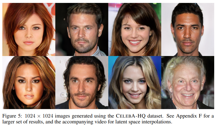
Our contributions allow us to deal with high output resolutions in a robust and efficient fashion. Figure 5 shows selected 1024 × 1024 images produced by our network.
While megapixel GAN results have been shown before in another dataset (Marchesi, 2017), our results are vastly more varied and of higher perceptual quality. Please refer to Appendix F for a larger set of result images as well as the nearest neighbors found from the training data.
The accompanying video shows latent space interpolations and visualizes the progressive training.
이를 위해 1024 × 1024 해상도에서 30000 개의 이미지로 구성된 CELEBA 데이터 세트의 고품질 버전을 만들었습니다.
이 데이터 세트 생성에 대한 자세한 내용은 부록 C를 참조하십시오.
우리의 기여를 통해 우리는 강력하고 효율적인 방식으로 높은 출력 해상도를 처리 할 수 있습니다.
그림 5는 네트워크에서 생성 된 1024 × 1024 이미지를 보여줍니다.
메가 픽셀 GAN 결과는 이전에 다른 데이터 세트 (Marchesi, 2017)에서 보여졌지만 우리의 결과는 훨씬 더 다양하고 지각 품질이 더 높습니다.
더 큰 결과 이미지 세트와 훈련 데이터에서 찾은 최근 접 이웃에 대해서는 부록 F를 참조하십시오.
The interpolation works so that we first randomize a latent code for each frame (512 components sampled individually from N (0, 1)), then blur the latents across time with a Gaussian (σ = 45 frames @ 60Hz), and finally normalize each vector to lie on a hypersphere.
We trained the network on 8 Tesla V100 GPUs for 4 days, after which we no longer observed qualitative differences between the results of consecutive training iterations.
Our implementation used an adaptive minibatch size depending on the current output resolution so that the available memory budget was optimally utilized.
In order to demonstrate that our contributions are largely orthogonal to the choice of a loss function, we also trained the same network using LSGAN loss instead of WGAN-GP loss. Figure 1 shows six examples of 10242 images produced using our method using LSGAN. Further details of this setup are given in Appendix B.
보간은 먼저 각 프레임 (N (0, 1)에서 개별적으로 샘플링 된 512 개의 구성 요소)에 대한 잠재 코드를 무작위 화 한 다음 가우시안 (σ = 45 프레임 @ 60Hz)을 사용하여 시간에 따라 잠재 성을 흐리게하고 마지막으로 각각을 정규화하도록 작동합니다.
벡터는 하이퍼 스피어에 있습니다. 우리는 4 일 동안 8 개의 Tesla V100 GPU에서 네트워크를 훈련 시켰으며, 그 후에는 더 이상 연속 훈련 반복 결과 간의 질적 차이를 관찰하지 않았습니다.
우리의 구현은 현재 출력 해상도에 따라 적응 형 미니 배치 크기를 사용하여 사용 가능한 메모리 예산을 최적으로 활용했습니다.
우리의 기여가 손실 함수 선택과 대체로 직교 함을 입증하기 위해 우리는 WGAN-GP 손실 대신 LSGAN 손실을 사용하여 동일한 네트워크를 훈련했습니다. 그림 1은 LSGAN을 사용한 방법을 사용하여 생성 된 10242 이미지의 여섯 가지 예를 보여줍니다. 이 설정에 대한 자세한 내용은 부록 B에 나와 있습니다.
6.4 LSUN RESULTS


Figure 6 shows a purely visual comparison between our solution and earlier results in LSUN BEDROOM.
Figure 7 gives selected examples from seven very different LSUN categories at 2562 .
A larger, non-curated set of results from all 30 LSUN categories is available in Appendix G, and the video demonstrates interpolations.
We are not aware of earlier results in most of these categories, and while some categories work better than others, we feel that the overall quality is high.
그림 6은 우리 솔루션과 LSUN BEDROOM의 이전 결과를 시각적으로 비교 한 것입니다.
그림 7은 2562의 7 개의 매우 다른 LSUN 범주에서 선택한 예를 보여줍니다.
30 개의 LSUN 범주 모두에서 선별되지 않은 더 큰 결과 세트는 부록 G에서 볼 수 있으며 비디오는 보간법을 보여줍니다.
대부분의 카테고리에서 이전 결과를 알지 못하며 일부 카테고리가 다른 카테고리보다 더 잘 작동하지만 전반적인 품질이 높다고 생각합니다.
6.5 CIFAR10 INCEPTION SCORES
The best inception scores for CIFAR10 (10 categories of 32 × 32 RGB images) we are aware of are 7.90 for unsupervised and 8.87 for label conditioned setups (Grinblat et al., 2017).
The large difference between the two numbers is primarily caused by “ghosts” that necessarily appear between classes in the unsupervised setting, while label conditioning can remove many such transitions.
When all of our contributions are enabled, we get 8.80 in the unsupervised setting.
Appendix D shows a representative set of generated images along with a more comprehensive list of results from earlier methods.
The network and training setup were the same as for CELEBA, progression limited to 32 × 32 of course.
The only customization was to the WGAN-GP’s regularization term Exˆ∼Pxˆ [(||∇xˆD(xˆ)||2 − γ) 2/γ2 ]. Gulrajani et al. (2017) used γ = 1.0, which corresponds to 1-Lipschitz, but we noticed that it is in fact significantly better to prefer fast transitions (γ = 750) to minimize the ghosts.
We have not tried this trick with other datasets.
우리가 알고있는 CIFAR10 (32 × 32 RGB 이미지의 10 개 범주)에 대한 최고 시작 점수는 감독되지 않은 경우 7.90이고 레이블 조정 설정의 경우 8.87입니다 (Grinblat et al., 2017).
두 숫자 사이의 큰 차이는 주로 감독되지 않은 설정에서 클래스간에 반드시 나타나는 "고스트"에 의해 발생하는 반면 레이블 컨디셔닝은 이러한 많은 전환을 제거 할 수 있습니다.
모든 기여가 활성화되면 감독되지 않은 설정에서 8.80을 얻습니다.
부록 D는 생성 된 이미지의 대표 세트와 이전 방법의보다 포괄적인 결과 목록을 보여줍니다.
네트워크 및 교육 설정은 CELEBA와 동일했으며 진행률은 물론 32 × 32로 제한되었습니다. 일한 사용자 정의는 WGAN-GP의 정규화 항 Exˆ∼Pxˆ [(|| ∇xˆD (xˆ) || 2 − γ) 2 / γ2]에 대한 것입니다.
Gulrajani et al. (2017)은 1-Lipschitz에 해당하는 γ = 1.0을 사용했지만 실제로는 고스트를 최소화하기 위해 빠른 전환 (γ = 750)을 선호하는 것이 훨씬 낫다는 것을 알았습니다. 우리는 다른 데이터 세트에서이 트릭을 시도하지 않았습니다.
7 DISCUSSION
While the quality of our results is generally high compared to earlier work on GANs, and the training is stable in large resolutions, there is a long way to true photorealism.
Semantic sensibility and understanding dataset-dependent constraints, such as certain objects being straight rather than curved, leaves a lot to be desired.
There is also room for improvement in the micro-structure of the images.
That said, we feel that convincing realism may now be within reach, especially in CELEBA-HQ.
결과의 품질은 일반적으로 GAN에 대한 이전 작업에 비해 높고 교육은 큰 해상도에서 안정적이지만 진정한 포토 리얼리즘에는 먼 길이 있습니다.
의미론적 감수성과 곡선이 아닌 직선인 특정 객체와 같은 데이터 세트 종속적 제약을 이해하는 것은 많이 필요합니다.
이미지의 미세 구조를 개선 할 여지도 있습니다.
즉, 우리는 특히 CELEBA-HQ에서 설득력있는 현실감이 이제 도달 할 수 있다고 생각합니다.
'비지도학습 > GAN' 카테고리의 다른 글
| AdaIN,2017 (0) | 2021.03.11 |
|---|---|
| Improved Training of Wasserstein GANs,2017 (0) | 2021.03.11 |
| [논문]StyleGAN,2019 (0) | 2021.03.10 |
| Analyzing and Improving the Image Quality of StyleGAN, 2020(StyleGAN2) (0) | 2021.03.02 |
| A Style-Based Generator Architecture for Generative Adversarial Networks, 2019(버전 1) (0) | 2021.03.02 |


