RetinaFace: Single-stage Dense Face Localisation in the Wild
Abstract
Though tremendous strides have been made in uncontrolled face detection, accurate and efficient face localisation in the wild remains an open challenge. This paper presents a robust single-stage face detector, named RetinaFace, which performs pixel-wise face localisation on various scales of faces by taking advantages of joint extra-supervised and self-supervised multi-task learning. Specifically, We make contributions in the following five aspects: (1) We manually annotate five facial landmarks on the WIDER FACE dataset and observe significant improvement in hard face detection with the assistance of this extra supervision signal. (2) We further add a selfsupervised mesh decoder branch for predicting a pixel-wise 3D shape face information in parallel with the existing supervised branches. (3) On the WIDER FACE hard test set, RetinaFace outperforms the state of the art average precision (AP) by 1.1% (achieving AP equal to 91.4%). (4) On the IJB-C test set, RetinaFace enables state of the art methods (ArcFace) to improve their results in face verification (TAR=89.59% for FAR=1e-6). (5) By employing light-weight backbone networks, RetinaFace can run real-time on a single CPU core for a VGA-resolution image. Extra annotations and code have been made available at: https://github.com/deepinsight/ insightface/tree/master/RetinaFace.
통제되지 않은 얼굴 감지 분야에서 엄청난 발전이 있었지만 야생에서 정확하고 효율적인 얼굴 위치 파악은 여전히 어려운 과제입니다.
이 논문은 RetinaFace라는 강력한 단일 단계 얼굴 감지기를 제시합니다.
RetinaFace는 관절 추가 감독 및 자체 감독 다중 작업 학습의 이점을 활용하여 다양한 얼굴 크기에서 픽셀 단위 얼굴 위치 파악을 수행합니다.
구체적으로 다음과 같은 5 가지 측면에서 기여합니다.
(1) WIDER FACE 데이터 세트에서 5 개의 얼굴 랜드 마크에 수동으로 주석을 달고이 추가 감독 신호의 도움으로 단단한 얼굴 감지의 상당한 개선을 관찰
(2) 기존의지도 브랜치와 병렬로 픽셀 단위의 3D 모양 얼굴 정보를 예측하기 위해 자체지도 메시 디코더 브랜치를 추가합니다.
(3) WIDER FACE 하드 테스트 세트에서 RetinaFace는 최첨단 평균 정밀도 (AP)보다 1.1 % (91.4 %에 해당하는 AP 달성) 성능이 뛰어납니다.
(4) IJB-C 테스트 세트에서 RetinaFace는 최첨단 방법 (ArcFace)을 사용하여 얼굴 확인 결과를 개선 할 수 있습니다 (FAR = 1e-6의 경우 TAR = 89.59 %). (5) 경량 백본 네트워크를 사용함으로써 RetinaFace는 VGA 해상도 이미지를 위해 단일 CPU 코어에서 실시간으로 실행할 수 있습니다.
추가 주석 및 코드는 https://github.com/deepinsight/insightface/tree/master/RetinaFace에서 사용할 수 있습니다.
1.Introduction
Automatic face localisation is the prerequisite step of facial image analysis for many applications such as facial attribute (e.g. expression [64] and age [38]) and facial identity recognition [45, 31, 55, 11]. A narrow definition of face localisation may refer to traditional face detection [53, 62], which aims at estimating the face bounding boxes without any scale and position prior. Nevertheless, in this paper we refer to a broader definition of face localisation which includes face detection [39], face alignment [13], pixelwise face parsing [48] and 3D dense correspondence regression [2, 12]. That kind of dense face localisation provides accurate facial position information for all different scales.
자동 얼굴 위치 파악은 얼굴 속성 (예 : 표정 [64] 및 나이 [38]) 및 얼굴 정체성 인식 [45, 31, 55, 11]과 같은 많은 응용 분야에서 얼굴 이미지 분석의 전제 조건입니다.
얼굴 위치 파악의 좁은 정의는 기존의 얼굴 감지 [53, 62]를 참조 할 수 있으며, 이는 사전에 스케일 및 위치없이 얼굴 경계 상자를 추정하는 것을 목표로 함.
그럼에도 불구하고, 이 논문에서 우리는 얼굴 검출 [39], 얼굴 정렬 [13], 픽셀 별 얼굴 분석 [48] 및 3D 밀집 대응 회귀(3D dense correspondence regression) [2, 12]를 포함하는 얼굴 위치 파악의 더 넓은 정의를 참조합니다.
이러한 종류의 조밀한 얼굴 위치 파악은 모든 다른 스케일에 대해 정확한 얼굴 위치 정보를 제공합니다.
Inspired by generic object detection methods [16, 43, 30, 41, 42, 28, 29], which embraced all the recent advances in deep learning, face detection has recently achieved remarkable progress [23, 36, 68, 8, 49]. Different from generic object detection, face detection features smaller ratio variations (from 1:1 to 1:1.5) but much larger scale variations (from several pixels to thousand pixels). The most recent state-of-the-art methods [36, 68, 49] focus on singlestage [30, 29] design which densely samples face locations and scales on feature pyramids [28], demonstrating promising performance and yielding faster speed compared to twostage methods [43, 63, 8]. Following this route, we improve the single-stage face detection framework and propose a state-of-the-art dense face localisation method by exploiting multi-task losses coming from strongly supervised and self-supervised signals. Our idea is examplified in Fig. 1.
최근 딥 러닝의 모든 발전을 포괄한 일반적인 물체 감지 방법 [16, 43, 30, 41, 42, 28, 29]에서 영감을 얻은 얼굴 인식은 최근 놀라운 발전을 이루었습니다
일반 물체 감지와는 달리 얼굴 감지는 비율 차이가 더 작지만, (1 : 1 ~ 1 : 1.5) 훨씬 더 큰 스케일 차이 (몇 픽셀에서 수천 픽셀)를 제공합니다.
가장 최근의 최첨단 방법 [36, 68, 49]은 단일 단계 [30, 29] 설계에 초점을 맞추고 있으며, 피처 피라미드에서면 위치와 스케일을 조밀하게 샘플링하여 [28], 유망한 성능을 보여주고 2 단계 방법과 비교하여 더 높은 속도 [43, 63, 8].
이 경로를 따라 우리는 단일 단계 얼굴 감지 프레임 워크를 개선하고 강력한 감독 및 자체 감독 신호(strongly supervised and self-supervised signals)에서 발생하는 다중 작업 손실을 활용하여 최첨단 조밀 얼굴 위치 파악 방법을 제안합니다.
우리의 아이디어는 그림 1에 예시되어 있습니다.
Typically, face detection training process contains both classification and box regression losses [16]. Chen et al. [6] proposed to combine face detection and alignment in a joint cascade framework based on the observation that aligned face shapes provide better features for face classification. Inspired by [6], MTCNN [66] and STN [5] simultaneously detected faces and five facial landmarks. Due to training data limitation, JDA [6], MTCNN [66] and STN [5] have not verified whether tiny face detection can benefit from the extra supervision of five facial landmarks. One of the questions we aim at answering in this paper is whether we can push forward the current best performance (90.3% [67]) on the WIDER FACE hard test set [60] by using extra supervision signal built of five facial landmarks.
일반적으로 얼굴 감지 훈련 과정에는 분류 및 상자 회귀 손실이 모두 포함됩니다 [16].
Chen et al. [6] 정렬 된 얼굴 모양이 얼굴 분류를위한 더 나은 기능을 제공한다는 관찰을 기반으로 공동 캐스케이드 프레임 워크에서 얼굴 감지 및 정렬을 결합하도록 제안했습니다.
[6], MTCNN [66] 및 STN [5]에서 영감을 받아 얼굴과 5 개의 얼굴 랜드 마크를 동시에 감지했습니다.
훈련 데이터 제한으로 인해 JDA [6], MTCNN [66] 및 STN [5]은 작은 얼굴 감지(tiny face detection)가 5 개의 얼굴 랜드 마크에 대한 추가 감독의 이점을 얻을 수 있는지 여부를 확인하지 않았습니다.
이 논문에서 우리가 답하고자하는 질문 중 하나는 5 개의 얼굴 랜드 마크로 구성된 추가 감독 신호를 사용하여 WIDER FACE 하드 테스트 세트 [60]에서 현재 최고의 성능 (90.3 % [67])을 추진할 수 있는지 여부입니다.
In Mask R-CNN [20], the detection performance is significantly improved by adding a branch for predicting an object mask in parallel with the existing branch for bounding box recognition and regression. That confirms that dense pixel-wise annotations are also beneficial to improve detection. Unfortunately, for the challenging faces of WIDER FACE it is not possible to conduct dense face annotation (either in the form of more landmarks or semantic segments). Since supervised signals cannot be easily obtained, the question is whether we can apply unsupervised methods to further improve face detection.
Mask R-CNN [20]에서는 기존의 바운딩박스 인식 및 회귀를 위한 분기(branch)와 병행하여 물체 마스크를 예측하기위한 분기를 추가함으로써 탐지 성능이 크게 향상되었습니다.
이는 조밀한 픽셀 단위 주석(dense pixel-wise annotations)도 탐지를 개선하는 데 도움이된다는 것을 확인합니다.
안타깝게도 WIDER FACE의 까다로운 얼굴의 경우 조밀한 얼굴 주석을 수행 할 수 없습니다 (더 많은 랜드 마크 또는 의미 세그먼트의 형태로).
감독 신호를 쉽게 얻을 수 없기 때문에 문제는 얼굴 감지를 더욱 향상시키기 위해 감독되지 않은 방법을 적용 할 수 있는지 여부입니다.
In FAN [56], an anchor-level attention map is proposed to improve the occluded face detection. Nevertheless, the proposed attention map is quite coarse and does not contain semantic information. Recently, self-supervised 3D morphable models [14, 51, 52, 70] have achieved promising 3D face modelling in-the-wild. Especially, Mesh Decoder [70] achieves over real-time speed by exploiting graph convolutions [10, 40] on joint shape and texture. However, the main challenges of applying mesh decoder [70] into the single-stage detector are: (1) camera parameters are hard to estimate accurately, and (2) the joint latent shape and texture representation is predicted from a single feature vector (1 × 1 Conv on feature pyramid) instead of the RoI pooled feature, which indicates the risk of feature shift.
In this paper, we employ a mesh decoder [70] branch through self-supervision learning for predicting a pixel-wise 3D face shape in parallel with the existing supervised branches. To summarise, our key contributions are:
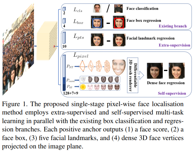
• Based on a single-stage design, we propose a novel pixel-wise face localisation method named RetinaFace, which employs a multi-task learning strategy to simultaneously predict face score, face box, five facial landmarks, and 3D position and correspondence of each facial pixel.
• On the WIDER FACE hard subset, RetinaFace outperforms the AP of the state of the art two-stage method (ISRN [67]) by 1.1% (AP equal to 91.4%).
• On the IJB-C dataset, RetinaFace helps to improve ArcFace’s [11] verification accuracy (with TAR equal to 89.59% when FAR=1e-6). This indicates that better face localisation can significantly improve face recognition.
• By employing light-weight backbone networks, RetinaFace can run real-time on a single CPU core for a VGA-resolution image.
• Extra annotations and code have been released to facilitate future research.
Face Attention Network(FAN) [56]에서는 가려진 얼굴 감지를 개선하기 위해 앵커 수준의 주의 맵(attention)이 제안되었습니다.
그럼에도 불구하고 제안 된 어텐션 맵은 매우 거칠고(coarse), 의미 정보를 포함하지 않습니다.
최근에는 자가지도 3D 모핑 모델(self-supervised 3D morphable models) [14, 51, 52, 70]이 유망한 3D 얼굴 모델링을 현장에서 달성했습니다.
특히, Mesh Decoder [70]는 관절 모양과 질감에 대한 그래프 convolution [10, 40]을 활용하여 실시간 이상의 속도를 달성합니다.
그러나 메시 디코더(Mesh Decoder) [70]를 단일 단계 검출기에 적용하는 주요 과제는 다음과 같습니다.
(1) 카메라 매개 변수를 정확하게 추정하기 어렵고
(2) 결합 잠재 형상 및 텍스처 표현이 단일 특징 벡터에서 예측됩니다 ( 1 × 1 Conv on feature pyramid), RoI 풀링 된 기능 대신, 기능 이동의 위험을 나타냅니다.
본 논문에서는 ✔기존의 지도 브랜치(existing supervised branches)와 병렬로 픽셀 단위의 3D 얼굴 모양을 예측하기 위해 자가 감독 학습✔을 통해 ✔메시 디코더 [70] 브랜치(mesh decoder [70] branch)✔를 사용합니다.
요약하자면 우리의 주요 기여는 다음과 같습니다.
• 단일 단계 설계를 기반으로 우리는 다중 작업 학습 전략(multi-task learning strategy)을 사용하여 얼굴 점수(face score), 얼굴 상자(face box), 5개의 얼굴 랜드 마크, 3D 위치 및 각각의 각 얼굴 픽셀에 해당하는 대응 관계를 동시에 예측하는 RetinaFace라는 새로운 픽셀 단위 얼굴 위치 파악 방법을 제안
• WIDER FACE 하드 서브 세트에서 RetinaFace는 최첨단 2 단계 방법 (ISRN [67])의 AP보다 1.1 % (AP는 91.4 %) 뛰어납니다.
• IJB-C 데이터 세트에서 RetinaFace는 ArcFace의 [11] 검증 정확도를 개선하는 데 도움이됩니다 (FAR = 1e-6 일 때 TAR은 89.59 % 임). 이것은 더 나은 얼굴 위치 파악이 얼굴 인식을 크게 향상시킬 수 있음을 나타냅니다.
• 가벼운 백본 네트워크를 사용함으로써 RetinaFace는 VGA 해상도 이미지를 위해 단일 CPU 코어에서 실시간으로 실행할 수 있습니다.
• 향후 연구를 용이하게하기 위해 추가 주석 및 코드가 릴리스되었습니다.
2. Related Work
Image pyramid v.s. feature pyramid: The slidingwindow paradigm, in which a classifier is applied on a dense image grid, can be traced back to past decades. The milestone work of Viola-Jones [53] explored cascade chain to reject false face regions from an image pyramid with real-time efficiency, leading to the widespread adoption of such scale-invariant face detection framework [66, 5]. Even though the sliding-window on image pyramid was the leading detection paradigm [19, 32], with the emergence of feature pyramid [28], sliding-anchor [43] on multi-scale feature maps [68, 49], quickly dominated face detection.
이미지 피라미드 대 피처 피라미드 : 분류기가 조밀한 이미지 그리드(dense image grid)에 적용되는 슬라이딩 윈도우 패러다임은 지난 수십 년으로 거슬러 올라갈 수 있습니다.
Viola-Jones [53]의 milestone work는 실시간 효율성으로 이미지 피라미드에서 거짓 얼굴 영역을 거부하는 캐스케이드 체인을 탐색하여 이러한 스케일 불변 얼굴 감지 프레임 워크를 널리 채택하게했습니다 [66, 5].
이미지 피라미드의 슬라이딩 윈도우가 주요 탐지 패러다임 [19, 32] 이었지만, 피쳐 피라미드 (Feature Pyramid),다중 스케일 피쳐 맵 [68, 49]의 슬라이딩 앵커 [43]의 등장으로 [28], 얼굴 검출쪽에서 빠르게 우세했습니다.
Two-stage v.s. single-stage: Current face detection methods have inherited some achievements from generic object detection approaches and can be divided into two categories: two-stage methods (e.g. Faster R-CNN [43, 63, 72]) and single-stage methods (e.g. SSD [30, 68] and RetinaNet [29, 49]). Two-stage methods employed a “proposal and refinement” mechanism featuring high localisation accuracy. By contrast, single-stage methods densely sampled face locations and scales, which resulted in extremely unbalanced positive and negative samples during training. To handle this imbalance, sampling [47] and re-weighting [29] methods were widely adopted. Compared to two-stage methods, single-stage methods are more efficient and have higher recall rate but at the risk of achieving a higher false positive rate and compromising the localisation accuracy.
Two-stage v.s. single-stage: 현재의 얼굴 감지 방법은 일반적인 물체 감지 접근 방식에서 일부 성과를 물려 왔으며 2 단계 방법 (예 : Faster R-CNN [43, 63, 72]) 및 단일 단계 방법 (예 : SSD [30, 68] 및 RetinaNet [29, 49]).
Two-stage는 높은 위치 정확도를 특징으로하는 "제안 및 개선"(“proposal and refinement”)메커니즘을 사용했습니다.
대조적으로, single-stage은 얼굴 위치와 척도를 조밀하게 샘플링하여 훈련 중에 극도로 불균형한 positive 및 negative 샘플을 생성했습니다.
이러한 불균형을 처리하기 위해 샘플링 [47] 및 재가중 [29] 방법(sampling [47] and re-weighting [29] methods)이 널리 채택되었습니다.
2 단계 방법에 비해 단일 단계 방법이 더 효율적이고 재현율이 더 높지만 ,더 높은 false-positive rate을 달성하고 현지화 정확도를 떨어 뜨릴 위험이 있습니다.
Context Modelling: To enhance the model’s contextual reasoning power for capturing tiny faces [23], SSH [36] and PyramidBox [49] applied context modules on feature pyramids to enlarge the receptive field from Euclidean grids. To enhance the non-rigid transformation modelling capacity of CNNs, deformable convolution network (DCN) [9, 74] employed a novel deformable layer to model geometric transformations. The champion solution of the WIDER Face Challenge 2018 [33] indicates that rigid (expansion) and non-rigid (deformation) context modelling are complementary and orthogonal to improve the performance of face detection.
컨텍스트 모델링(Context Modelling) : 작은 얼굴을 캡처하기위한 모델의 컨텍스트 추론 능력을 향상시키기 위해 [23], SSH [36] 및 PyramidBox [49]는 피처 피라미드(Feature Pyramid)에 컨텍스트 모듈을 적용하여 유클리드 그리드(Euclidean grids)의 수용 필드(Receptive Field)를 확대했습니다.
CNN의 비강성 변환 모델링 능력(non-rigid transformation modelling capacity)을 향상시키기 위해 변형 가능한 컨볼루션 네트워크 (DCN) [9, 74]는 기하 변환을 모델링하기 위해 새로운 변형 가능한 레이어를 사용했습니다.
WIDER Face Challenge 2018 [33]의 챔피언 솔루션은 강체 (확장) 및 비 강체 (변형) 컨텍스트 모델링이 얼굴 감지 성능을 향상시키기 위해 상호 보완적이고 직교 함을 나타냅니다.
Multi-task Learning: Joint face detection and alignment is widely used [6, 66, 5] as aligned face shapes provide better features for face classification. In Mask R-CNN [20], the detection performance was significantly improved by adding a branch for predicting an object mask in parallel with the existing branches. Densepose [1] adopted the architecture of Mask-RCNN to obtain dense part labels and coordinates within each of the selected regions. Nevertheless, the dense regression branch in [20, 1] was trained by supervised learning. In addition, the dense branch was a small FCN applied to each RoI to predict a pixel-to-pixel dense mapping.
멀티 태스킹 학습(Multi-task Learning) :
정렬된 얼굴 모양이 얼굴 분류에 더 나은 기능을 제공하기 때문에 관절 얼굴 감지 및 정렬이 널리 사용됩니다 [6, 66, 5].
Mask R-CNN [20]에서는 기존 분기와 병렬로 객체 마스크를 예측하기위한 분기(branch)를 추가하여 탐지 성능이 크게 향상되었습니다.
DensePose [1]은 Mask-RCNN의 아키텍처를 채택하여 선택한 각 영역 내에서 조밀한 부품 레이블과 좌표를 얻었습니다.
그럼에도 불구하고 [20, 1]의 고밀도 회귀 분기(dense regression branch)는 지도 학습으로 훈련되었습니다.
또한, 고밀도 브랜치는 픽셀 대 픽셀 고밀도 매핑(pixel-to-pixel dense mapping)을 예측하기 위해 각 RoI에 적용된 작은 FCN이었습니다.
3. RetinaFace

3.1. Multi-task Loss 다중 작업 손실
For any training anchor i, we minimise the following multi-task loss: L = Lcls(pi , p∗ i ) + λ1p ∗ i Lbox(ti , t∗ i ) + λ2p ∗ i Lpts(li , l∗ i ) + λ3p ∗ i Lpixel. (1) (1) Face classification loss Lcls(pi , p∗ i ), where pi is the predicted probability of anchor i being a face and p ∗ i is 1 for the positive anchor and 0 for the negative anchor. The classification loss Lcls is the softmax loss for binary classes (face/not face). (2) Face box regression loss Lbox(ti , t∗ i ), where ti = {tx, ty, tw, th}i and t ∗ i = {t ∗ x , t∗ y , t∗ w, t∗ h }i represent the coordinates of the predicted box and ground-truth box associated with the positive anchor. We follow [16] to normalise the box regression targets (i.e. centre location, width and height) and use Lbox(ti , t∗ i ) = R(ti − t ∗ i ), where R is the robust loss function (smooth-L1) defined in [16]. (3) Facial landmark regression loss Lpts(li , l∗ i ), where li = {lx1 , ly1 , . . . , lx5 , ly5 }i and l ∗ i = {l ∗ x1 , l∗ y1 , . . . , l∗ x5 , l∗ y5 }i represent the predicted five facial landmarks and groundtruth associated with the positive anchor. Similar to the box centre regression, the five facial landmark regression also employs the target normalisation based on the anchor centre. (4) Dense regression loss Lpixel (refer to Eq. 3). The loss-balancing parameters λ1-λ3 are set to 0.25, 0.1 and 0.01, which means that we increase the significance of better box and landmark locations from supervision signals.
모든 훈련 앵커 i에 대해 다음과 같은 다중 작업 손실을 최소화합니다 .
(1) 얼굴 분류 손실 $L_{cls}(p_i,p^∗_i)$, 여기서 $p_i$는 앵커 i가 얼굴이 될 것으로 예상되는 확률이고,
$p^∗_i$는 양의 앵커의 경우 1이고 음의 앵커의 경우 0입니다.
분류 손실 $L_{cls}$는 이진 클래스 (얼굴 / 얼굴 아님)에 대한 소프트 맥스 손실입니다.
(2) 페이스 박스 회귀 손실 $L_{box}(t_i,t^∗_i)$, 여기서 $t_i={t_x,t_y,t_w,t_h}_i$ 및 $t^∗_i={t^∗_x,t^∗_y,t^∗_w,t^∗_h}_i$는 포지티브 앵커와 관련된 예측 상자와 실측 상자의 좌표를 나타냅니다.
바운딩박스 회귀 목적함수(Boundingbox regression objective) (즉, 중심 위치, 너비 및 높이)를 정규화하기 위해 [16]을 따르고
$L_{box}(t_i,t^∗_i)=R(t_i−t^∗_i)$를 사용합니다.
여기서 R은 로버스트 손실 함수 (smooth- L1)는 [16]에 정의되어 있습니다.
(3) 얼굴 랜드 마크 회귀 손실 $L_{pts}(l_i,l^∗_i)$, 여기서 $l_i={l_{x1},l_{y1},. . . ,l_{x5},l_{y5}}_i$ 및 $l^∗_i={l^∗_{x1},l^∗_{y1},. . . ,l^*_{x5},l^*_{y5}}_i$는 포지티브 앵커와 관련된 예측 된 5 개의 얼굴 랜드 마크와 근거를 나타냅니다.
상자 중심 회귀(Box center regression)와 유사하게, 5 개의 얼굴 랜드 마크 회귀는 앵커 중심을 기반으로하는 대상 정규화를 사용합니다.
(4) Dense regression loss $L_{pixel}$ (Eq. 3 참조). 손실 균형 매개 변수 $λ1-λ3$은 0.25, 0.1 및 0.01로 설정되어 있으며, 이는 감독 신호에서 더 나은 상자 및 랜드 마크 위치의 중요성을 증가 시킨다는 것을 의미합니다.
3.2. Dense Regression Branch 고밀도 회귀 분기
Mesh Decoder. 메시 디코더.
We directly employ the mesh decoder (mesh convolution and mesh up-sampling) from [70, 40], which is a graph convolution method based on fast localised spectral filtering [10]. In order to achieve further acceleration, we also use a joint shape and texture decoder similarly to the method in [70], contrary to [40] which only decoded shape.
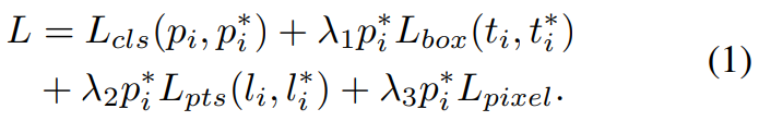
Below we will briefly explain the concept of graph convolutions and outline why they can be used for fast decoding. As illustrated in Fig. 3(a), a 2D convolutional operation is a “kernel-weighted neighbour sum” within the Euclidean grid receptive field. Similarly, graph convolution also employs the same concept as shown in Fig. 3(b). However, the neighbour distance is calculated on the graph by counting the minimum number of edges connecting two vertices. We follow [70] to define a coloured face mesh G = (V, E), where V ∈ R n×6 is a set of face vertices containing the joint shape and texture information, and E ∈ {0, 1} n×n is a sparse adjacency matrix encoding the connection status between vertices. The graph Laplacian is defined as L = D − E ∈ R n×n where D ∈ R n×n is a diagonal matrix with Dii = P j Eij .
우리는 [70, 40]의 메시 디코더 (메시 컨볼루션 및 메시 업샘플링)를 직접 사용하는데, 이는 빠른 국소 스펙트럼 필터링(fast localised spectral filtering)에 기반한 그래프 컨볼루션 방법임
추가 가속(further acceleration)을 달성하기 위해, 우리는 또한 [70]의 방법과 유사한 조인트 모양 및 텍스처 디코더(joint shape and texture decoder)를 사용합니다.
[40]와 다르게 모양만 디코딩했습니다.
아래에서는 그래프 컨볼루션의 개념을 간략하게 설명하고 빠른 디코딩에 사용할 수있는 이유를 간략하게 설명합니다.
그림 3 (a)에서 볼 수 있듯이 2D 컨볼 루션 연산은 유클리드 그리드 수용 필드 내에서 "커널 가중치 이웃 합"(“kernel-weighted neighbour sum”)입니다.
마찬가지로 그래프 컨볼루션도 그림 3 (b)에 표시된 것과 동일한 개념을 사용합니다.
그러나 인접 거리는 두 꼭지점을 연결하는 최소 가장자리 수를 계산하여 그래프에서 계산됩니다.
우리는 [70]에 따라 컬러면 메쉬 G = (V, E)를 정의합니다.
여기서 V ∈ R n × 6은 관절 모양과 텍스처 정보를 포함하는 얼굴 정점(face vertices) 세트이고,
E ∈ {0, 1} n × n은 정점 간의 연결 상태를 인코딩하는 희소 인접 행렬(sparse adjacency matrix).
그래프 Laplacian은 $L=D−E∈R^{n×n}$으로 정의됩니다. 여기서 $D∈R^{n×n}$은 $D_{ii}=\sum_jE_{ij}$ 인 대각 행렬입니다.
Following [10, 40, 70], the graph convolution with kernel gθ can be formulated as a recursive Chebyshev polynomial truncated at order K, y = gθ(L)x = K X−1 k=0 θkTk(L˜)x, (2) where θ ∈ R K is a vector of Chebyshev coefficients and Tk(L˜) ∈ R n×n is the Chebyshev polynomial of order k evaluated at the scaled Laplacian L˜. Denoting x¯k = Tk(L˜)x ∈ R n, we can recurrently compute x¯k = 2L˜x¯k−1− x¯k−2 with x¯0 = x and x¯1 = Lx˜ . The whole filtering operation is extremely efficient including K sparse matrix-vector multiplications and one dense matrix-vector multiplication y = gθ(L)x = [¯x0, . . . , x¯K−1]θ.
[10, 40, 70]에 따라 커널 $g_θ$가 있는 그래프 컨볼루션은 순서 K에서 잘린 재귀 체비 쇼프 다항식으로 공식화 될 수 있습니다

(2) $y=g_θ(L)x=\sum^{K-1}_{k=0}θ_kT_k(L^~)x$
여기서 $θ∈R^K$는 체비 쇼프 계수(Chebyshev coefficients)의 벡터이고,
$T_k(L^~)∈R^{n×n}$은 스케일링된 라플라시안 $L^~$에서 평가된 $k$차의 체비 쇼프 다항식(Chebyshev polynomial)입니다.
$x^¯_k=T_k(L^~)x∈R^n$으로 표시하면 $x^¯_0=x$ 및 $x^¯_1=L^~x$로 $x^¯_k=2L^~x^¯_{k-1}-x^¯_{k-2}$를 반복적으로 계산할 수 있습니다.
K개의 희소 행렬-벡터 곱셈(K sparse matrix-vector multiplications)과 하나의 조밀한 행렬-벡터 곱셈(dense matrix-vector multiplication) $y=g_θ(L)x=[x^¯_0,. . . , x^¯_{K-1}]θ$.
Differentiable Renderer. 차별화 가능한 렌더러.
After we predict the shape and texture parameters PST ∈ R 128, we employ an efficient differentiable 3D mesh renderer [14] to project a colouredmesh DPST onto a 2D image plane with camera parameters Pcam = [xc, yc, zc, x0 c , y0 c , z0 c , fc] (i.e. camera location, camera pose and focal length) and illumination parameters Pill = [xl , yl , zl , rl , gl , bl , ra, ga, ba] (i.e. location of point light source, colour values and colour of ambient lighting).
모양 및 텍스처 매개 변수 $P_{ST}∈R^128$을 예측한 후, 효율적으로 차별화 가능한 3D 메시 렌더러(3d mesh renderer) [14]를 사용하여 카메라 매개 변수 $P_{cam} = [x_c,y_c,z_c,x'_c,y'_c,z'_c,f_c]$을 사용하여 2D 이미지 평면에 컬러 메시 DPST를 투영합니다.
(즉, 카메라 위치, 카메라 포즈 및 초점 거리) 및 조명 매개 변수 $P_{ill}=[x_l, y_l, z_l, r_l, g_l, b_l, r_a, g_a, b_a]$ (즉, 포인트 광원의 위치, 색상 값 및 주변 조명 색상).
Dense Regression Loss. 고밀도 회귀 손실.
Once we get the rendered 2D face R(DPST , Pcam, Pill), we compare the pixel-wise difference of the rendered and the original 2D face using the following function: Lpixel = 1 W ∗ H X W i X H j kR(DPST , Pcam, Pill)i,j−I ∗ i,jk1, (3) where W and H are the width and height of the anchor crop I ∗ i,j , respectively.
렌더링된 2D 얼굴 R(D_{PST},P_{cam},P_{ill})을 얻으면 다음 함수를 사용하여 렌더링 된 2D 얼굴과 원래 2D 얼굴의 픽셀 단위 차이를 비교합니다.
(3) $L_{pixel}=fraciont{1}{W∗H}\sumW_i\sum^H_j ||R(D_{P_{ST}},P_{cam},P_{ill})_{i, j}−I^∗_{i, j}||_1$
여기서 W와 H는 각각 anchor crop $I^∗_{i, j}$의 너비와 높이입니다.
4. Experiments
4.1. Dataset
The WIDER FACE dataset [60] consists of 32, 203 images and 393, 703 face bounding boxes with a high degree of variability in scale, pose, expression, occlusion and illumination. The WIDER FACE dataset is split into training (40%), validation (10%) and testing (50%) subsets by randomly sampling from 61 scene categories. Based on the detection rate of EdgeBox [76], three levels of difficulty (i.e. Easy, Medium and Hard) are defined by incrementally incorporating hard samples.
WIDER FACE 데이터 셋 [60]은 32, 203 개의 이미지와 393, 703 개의 얼굴 경계 상자로 구성되며 스케일, 포즈, 표현, 오클루전 및 조명이 매우 다양. WIDER FACE 데이터 세트는 61 개의 장면 범주에서 무작위로 샘플링하여 훈련 (40 %), 검증 (10 %) 및 테스트 (50 %) 하위 집합으로 나뉩니다.
EdgeBox [76]의 탐지율에 따라 하드 샘플을 점진적으로 통합하여 세 가지 난이도 (즉, Easy, Medium 및 Hard)를 정의합니다.
Extra Annotations. 추가 주석.


As illustrated in Fig. 4 and Tab. 1, we define five levels of face image quality (according to how difficult it is to annotate landmarks on the face) and annotate five facial landmarks (i.e. eye centres, nose tip and mouth corners) on faces that can be annotated from the WIDER FACE training and validation subsets. In total, we have annotated 84.6k faces on the training set and 18.5k faces on the validation set.
그림 4와 Tab. 1, 얼굴 이미지 품질의 5단계를 정의하고 (얼굴의 랜드 마크에 주석을 달기가 얼마나 어려운지에 따라) WIDER FACE 학습 및 검증 서브 세트에서 주석을 달 수있는 얼굴에 5 개의 얼굴 랜드 마크 (예 : 눈 중앙, 코끝 및 입 모서리)에 주석을 답니다.
총 84.6k 개의 얼굴을 훈련 세트에, 18.5k 개의 얼굴을 검증 세트에 주석으로 달았습니다.
4.2. Implementation details
Feature Pyramid.
RetinaFace employs feature pyramid levels from P2 to P6, where P2 to P5 are computed from the output of the corresponding ResNet residual stage (C2 through C5) using top-down and lateral connections as in [28, 29]. P6 is calculated through a 3×3 convolution with stride=2 on C5. C1 to C5 is a pre-trained ResNet-152 [21] classification network on the ImageNet-11k dataset while P6 are randomly initialised with the “Xavier” method [17].
RetinaFace는 $P_2$에서 $P_6$까지의 피처 피라미드 레벨을 사용합니다.
여기서 $P_2$에서 $P_5$는 [28, 29]에서와 같이 하향식 및 측면 연결을 사용하여 해당 ResNet 잔여 단계 ($C_2$에서 $C_5$)의 출력에서 계산됩니다.
$P_6$은 $C_5$에서 stride = 2 인 3x3 컨볼 루션을 통해 계산됩니다.
$C_1$ ~ $C_5$는 ImageNet-11k 데이터 세트에 대한 사전 훈련 된 ResNet-152 [21] 분류 네트워크이며 P6은 "Xavier"방법 [17]으로 무작위로 초기화됩니다.
Context Module. 컨텍스트 모듈.
Inspired by SSH [36] and PyramidBox [49], we also apply independent context modules on five feature pyramid levels to increase the receptive field and enhance the rigid context modelling power. Drawing lessons from the champion of the WIDER Face Challenge 2018 [33], we also replace all 3 × 3 convolution layers within the lateral connections and context modules by the deformable convolution network (DCN) [9, 74], which further strengthens the non-rigid context modelling capacity.
SSH [36] 및 PyramidBox [49]에서 영감을 받아 5가지 기능 피라미드 수준에 독립적인 컨텍스트 모듈을 적용하여 수용 필드를 높이고 엄격한 컨텍스트 모델링 능력을 향상시킵니다.
WIDER Face Challenge 2018 [33]의 챔피언으로부터 교훈을 얻었으며 측면 연결 및 컨텍스트 모듈(lateral connections and context modules) 내의 모든 3×3 컨볼 루션 레이어를 비 -엄격한 컨텍스트 모델링 능력(non-rigid context modelling capacity)를 강화하는 DCN( deformable convolution network 변형 컨볼 루션 네트워크) [9, 74]으로 대체한다.
Loss Head.
For negative anchors, only classification loss is applied. For positive anchors, the proposed multi-task loss is calculated. We employ a shared loss head (1 × 1 conv) across different feature maps Hn × Wn × 256, n ∈ {2, . . . , 6}. For the mesh decoder, we apply the pre-trained model [70], which is a small computational overhead that allows for efficient inference.
네거티브 앵커의 경우 분류 손실만 적용됩니다.
포지티브 앵커의 경우 제안된 다중 작업 손실이 계산됩니다.
우리는 서로 다른 피처 맵 $H_n×W_n×256, n∈{2,. . . , 6}.$에서 공유 손실 헤드(shared loss head) (1 × 1 conv)를 사용합니다
메시 디코더의 경우, 효율적인 추론을 허용하는 작은 계산 오버 헤드인 사전 훈련된 모델 [70]을 적용합니다.
Anchor Settings. 앵커 설정.

As illustrated in Tab. 2, we employ scalespecific anchors on the feature pyramid levels from P2 to P6 like [56]. Here, P2 is designed to capture tiny faces by tiling small anchors at the cost of more computational time and at the risk of more false positives. We set the scale step at 2 1/3 and the aspect ratio at 1:1. With the input image size at 640 × 640, the anchors can cover scales from 16 × 16 to 406 × 406 on the feature pyramid levels. In total, there are 102,300 anchors, and 75% of these anchors are from P2. During training, anchors are matched to a ground-truth box when IoU is larger than 0.5, and to the background when IoU is less than 0.3. Unmatched anchors are ignored during training. Since most of the anchors (> 99%) are negative after the matching step, we employ standard OHEM [47, 68] to alleviate significant imbalance between the positive and negative training examples. More specifically, we sort negative anchors by the loss values and select the top ones so that the ratio between the negative and positive samples is at least 3:1.
Tab. 2에 설명 된대로, 우리는 [56]과 같이 $P_2$에서 $P_6$까지 피처 피라미드 레벨에 스케일 특정 앵커를 사용합니다.
여기에서 $P_2$는 더 많은 계산 시간과 더 많은 오탐의 위험이있는 작은 앵커를 타일링하여 작은 얼굴을 캡처하도록 설계되었습니다.
스케일 단계를 $2fraction{1}{3}$로 설정하고 종횡비를 1 : 1로 설정했습니다.
입력 이미지 크기가 640 × 640 인 경우 앵커는 피처 피라미드 수준에서 16 × 16에서 406 × 406까지의 배율을 포함 할 수 있습니다.
총 102,300 개의 앵커가 있으며, 이 앵커의 75%는 $P_2$에서 제공됩니다.
학습 중에 앵커는 IoU가 0.5보다 크면 Ground-Truth 상자에, IoU가 0.3보다 작으면 배경에 일치합니다.
학습 중에 일치하지 않는 앵커는 무시됩니다.
대부분의 앵커 (>99 %)는 매칭 단계 후에 음수이므로 표준 OHEM [47, 68]을 사용하여 양성 및 음성 학습 예제 간의 상당한 불균형을 완화합니다.
보다 구체적으로, 손실 값을 기준으로 negative anchor를 정렬하고 negative의 샘플과 positive의 샘플 간의 비율이 최소 3 : 1이되도록 상위 앵커를 선택합니다.
Data Augmentation.
Since there are around 20% tiny faces in the WIDER FACE training set, we follow [68, 49] and randomly crop square patches from the original images and resize these patches into 640 × 640 to generate larger training faces. More specifically, square patches are cropped from the original image with a random size between [0.3, 1] of the short edge of the original image. For the faces on the crop boundary, we keep the overlapped part of the face box if its centre is within the crop patch. Besides random crop, we also augment training data by random horizontal flip with the probability of 0.5 and photo-metric colour distortion [68].
WIDER FACE 트레이닝 세트에는 약 20 %의 작은 얼굴이 있으므로 [68, 49]를 따라 원본 이미지에서 정사각형 패치를 무작위로 자르고이 패치의 크기를 640 × 640으로 조정하여 더 큰 트레이닝 얼굴을 생성합니다.
보다 구체적으로, 정사각형 패치는 원본 이미지의 짧은 가장자리의 [0.3, 1] 사이에서 임의의 크기로 원본 이미지에서 잘립니다.
자르기 경계에있는면의 경우 가운데가 자르기 패치 내에 있으면 얼굴 박스의 겹친 부분을 유지합니다.
Random crop외에도 0.5의 확률과 photo-metric colour distortion[68]의 확률로 무작위 수평 뒤집기로 학습 데이터를 증가시킵니다.
Training Details.
We train the RetinaFace using SGD optimiser (momentum at 0.9, weight decay at 0.0005, batch size of 8 × 4) on four NVIDIA Tesla P40 (24GB) GPUs. The learning rate starts from 10−3 , rising to 10−2 after 5 epochs, then divided by 10 at 55 and 68 epochs. The training process terminates at 80 epochs.
4 개의 NVIDIA Tesla P40 (24GB) GPU에서 SGD 옵티 마이저 (모멘텀 0.9, 무게 감소 0.0005, 배치 크기 8 × 4)를 사용하여 RetinaFace를 훈련합니다. 학습률은 10−3에서 시작하여 5 epoch 후에 10−2로 상승한 다음 55 및 68 epoch에서 10으로 나뉩니다.
훈련 프로세스는 80 Epoch에서 종료됩니다.
Testing Details.
For testing on WIDER FACE, we follow the standard practices of [36, 68] and employ flip as well as multi-scale (the short edge of image at [500, 800, 1100, 1400, 1700]) strategies. Box voting [15] is applied on the union set of predicted face boxes using an IoU threshold at 0.4.
WIDER FACE에서 테스트하기 위해 우리는 [36, 68]의 표준 관행을 따르고 플립 및 다중 스케일 ([500, 800, 1100, 1400, 1700]에서 이미지의 짧은 가장자리) 전략을 사용합니다.
상자 투표(Box voting)[15]는 0.4에서 IoU 임계값을 사용하여 예측된 얼굴 상자의 IoU에 적용됩니다.
4.3. Ablation Study
To achieve a better understanding of the proposed RetinaFace, we conduct extensive ablation experiments to examine how the annotated five facial landmarks and the proposed dense regression branch quantitatively affect the performance of face detection. Besides the standard evaluation metric of average precision (AP) when IoU=0.5 on the Easy, Medium and Hard subsets, we also make use of the development server (Hard validation subset) of the WIDER Face Challenge 2018 [33], which employs a more strict evaluation metric of mean AP (mAP) for IoU=0.5:0.05:0.95, rewarding more accurate face detectors.
제안된 RetinaFace를 더 잘 이해하기 위해 우리는 주석이 달린 5개의 얼굴 랜드 마크와 제안된 고밀도 회귀 분기(Dense Regression Branch)가 얼굴 감지 성능에 정량적으로 영향을 미치는 방식을 조사하기 위해 광범위한 절제 실험을 수행합니다.
Easy, Medium 및 Hard 하위 집합에서 IoU = 0.5 일 때 평균 정밀도 (AP)의 표준 평가 메트릭 외에도 WIDER Face Challenge 2018 [33]의 개발 서버 (하드 유효성 검사 하위 집합)를 사용합니다.
IoU = 0.5 : 0.05 : 0.95에 대한 평균 AP(mAP)에 대한보다 엄격한 평가 메트릭을 사용하여보다 정확한 얼굴 감지기를 제공합니다.

As illustrated in Tab. 3, we evaluate the performance of several different settings on the WIDER FACE validation set and focus on the observations of AP and mAP on the Hard subset. By applying the practices of state-of-the-art techniques (i.e. FPN, context module, and deformable convolution), we set up a strong baseline (91.286%), which is slightly better than ISRN [67] (90.9%). Adding the branch of five facial landmark regression significantly improves the face box AP (0.408%) and mAP (0.775%) on the Hard subset, suggesting that landmark localisation is crucial for improving the accuracy of face detection. By contrast, adding the dense regression branch increases the face box AP on Easy and Medium subsets but slightly deteriorates the results on the Hard subset, indicating the difficulty of dense regression under challenging scenarios. Nevertheless, learning landmark and dense regression jointly enables a further improvement compared to adding landmark regression only. This demonstrates that landmark regression does help dense regression, which in turn boosts face detection performance even further.
Tab. 3에 설명 된대로, 우리는 WIDER FACE 검증 세트에서 여러 다른 설정의 성능을 평가하고 Hard 하위 세트에서 AP 및 mAP의 관찰에 중점을 둡니다. 최첨단 기술 (예 : FPN, 컨텍스트 모듈 및 변형 가능한 컨볼 루션)의 관행을 적용하여 강력한 기준선 (91.286 %)을 설정했습니다.
이는 ISRN [67] (90.9 %)보다 약간 낫습니다.
5 개의 얼굴 랜드 마크 회귀의 분기를 추가하면 하드 하위 집합에서 얼굴 상자 AP (0.408 %) 및 mAP (0.775 %)가 크게 향상되어 랜드 마크 위치 지정이 얼굴 감지의 정확도를 향상시키는 데 중요함을 시사합니다.
대조적으로 조밀 회귀 분기를 추가하면 Easy 및 Medium 하위 집합에서 페이스 박스 AP가 증가하지만 Hard 하위 집합의 결과가 약간 저하되어 까다로운 시나리오에서 조밀 회귀의 어려움을 나타냅니다.
그럼에도 불구하고 랜드 마크와 조밀 회귀를 공동으로 학습하면 랜드 마크 회귀 만 추가하는 것에 비해 추가 개선이 가능합니다.
이는 랜드 마크 회귀가 조밀한 회귀(dense regression)에 도움이되며, 이는 얼굴 감지 성능을 더욱 향상 시킨다는 것을 보여줍니다.
4.4. Face box Accuracy 페이스 박스 정확도

Following the stander evaluation protocol of the WIDER FACE dataset, we only train the model on the training set and test on both the validation and test sets. To obtain the evaluation results on the test set, we submit the detection results to the organisers for evaluation. As shown in Fig. 5, we compare the proposed RetinaFace with other 24 state-of-the-art face detection algorithms (i.e. Multiscale Cascade CNN [60], Two-stage CNN [60], ACFWIDER [58], Faceness-WIDER [59], Multitask Cascade CNN [66], CMS-RCNN [72], LDCF+ [37], HR [23], Face R-CNN [54], ScaleFace [61], SSH [36], SFD [68], Face RFCN [57], MSCNN [4], FAN [56], Zhu et al. [71], PyramidBox [49], FDNet [63], SRN [8], FANet [65], DSFD [27], DFS [50], VIM-FD [69], ISRN [67]). Our approach outper forms these state-of-the-art methods in terms of AP. More specifically, RetinaFace produces the best AP in all subsets of both validation and test sets, i.e., 96.9% (Easy), 96.1% (Medium) and 91.8% (Hard) for validation set, and 96.3% (Easy), 95.6% (Medium) and 91.4% (Hard) for test set. Compared to the recent best performed method [67], RetinaFace sets up a new impressive record (91.4% v.s. 90.3%) on the Hard subset which contains a large number of tiny faces.
WIDER FACE 데이터 세트의 표준 평가 프로토콜에 따라 훈련 세트에서만 모델을 훈련하고 검증 및 테스트 세트 모두에서 테스트합니다.
테스트 세트에 대한 평가 결과를 얻기 위해 평가를 위해 주최자에게 탐지 결과를 제출합니다.
그림 5에서 볼 수 있듯이 제안 된 RetinaFace를 다른 24 개의 최신 얼굴 감지 알고리즘 (예 : Multiscale Cascade CNN [60], Two-stage CNN [60], ACFWIDER [58], Faceness-WIDER)과 비교합니다.
[59], 멀티 태스킹 캐스케이드 CNN [66], CMS-RCNN [ 72], LDCF + [37], HR [23], Face R-CNN [54], ScaleFace [61], SSH [36], SFD [68] , Face RFCN [57], MSCNN [4], FAN [56], Zhu et al. [71], PyramidBox [49], FDNet [63], SRN [8], FANet [65], DSFD [27], DFS [50], VIM-FD [69], ISRN [67]).
우리의 접근 방식은 AP 측면에서 이러한 최첨단 방법을 능가합니다.
보다 구체적으로, RetinaFace는 검증 및 테스트 세트의 모든 하위 집합에서 최고의 AP를 생성합니다.
즉, 검증 세트의 경우 96.9 % (쉬움), 96.1 % (중간) 및 91.8 % (어려움), 96.3 % (쉬움), 95.6 % 테스트 세트의 경우 (중간) 및 91.4 % (하드).
RetinaFace는 최근 가장 잘 수행 된 방법 [67]과 비교하여 많은 수의 작은 얼굴을 포함하는 Hard 하위 집합에서 새로운 인상적인 기록 (91.4 % 대 90.3 %)을 설정했습니다.
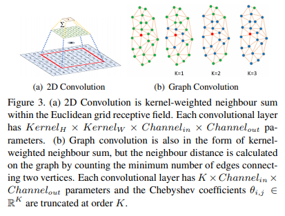
In Fig. 6, we illustrate qualitative results on a selfie with dense faces. RetinaFace successfully finds about 900 faces (threshold at 0.5) out of the reported 1, 151 faces. Besides accurate bounding boxes, the five facial landmarks predicted by RetinaFace are also very robust under the variations of pose, occlusion and resolution. Even though there are some failure cases of dense face localisation under heavy occlusion, the dense regression results on some clear and large faces are good and even show expression variations.
그림 6에서는 얼굴이 빽빽한 셀카의 질적 결과를 보여줍니다.
RetinaFace는보고 된 1,151 개의 얼굴 중 약 900 개의 얼굴 (0.5에서 임계 값)을 성공적으로 찾습니다.
정확한 경계 상자 외에도 RetinaFace에서 예측한 5 가지 얼굴 랜드 마크는 포즈, 폐색 및 해상도의 변화에서도 매우 강력합니다.
심한 폐색에서 조밀한 얼굴 국소화의 실패 사례가 있지만, 일부 명확하고 큰 얼굴에 대한 조밀한 회귀 결과가 좋고 심지어 표현 변화를 보여줍니다.
4.5. Five Facial Landmark Accuracy 5 가지 얼굴 랜드 마크 정확도

To evaluate the accuracy of five facial landmark localisation, we compare RetinaFace with MTCNN [66] on the AFLW dataset [26] (24,386 faces) as well as the WIDER FACE validation set (18.5k faces). Here, we employ the face box size (√ W × H) as the normalisation distance. As shown in Fig. 7(a), we give the mean error of each facial landmark on the AFLW dataset [73]. RetinaFace significantly decreases the normalised mean errors (NME) from 2.72% to 2.21% when compared to MTCNN. In Fig. 7(b), we show the cumulative error distribution (CED) curves on the WIDER FACE validation set. Compared to MTCNN, RetinaFace significantly decreases the failure rate from 26.31% to 9.37% (the NME threshold at 10%).
5 개의 얼굴 랜드 마크 위치 파악의 정확도를 평가하기 위해 RetinaFace를 AFLW 데이터 세트 [26] (24,386 개 얼굴) 및 WIDER FACE 검증 세트 (18.5k 얼굴)에서 MTCNN [66]과 비교합니다.
여기서는 정규화 거리로 페이스 박스 크기 $(\sqrt[W×H]{})$를 사용합니다.
그림 7 (a)에서 볼 수 있듯이 AFLW 데이터 셋에서 각 얼굴 랜드 마크의 평균 오차를 제공합니다 [73].
RetinaFace는 MTCNN과 비교할 때 정규화 된 평균 오차 (NME)를 2.72 %에서 2.21 %로 크게 줄입니다.
그림 7 (b)에서는 WIDER FACE 검증 세트의 누적 오차 분포 (CED) 곡선을 보여줍니다.
MTCNN과 비교하여 RetinaFace는 실패율을 26.31 %에서 9.37 % (10 %에서 NME 임계 값)로 크게 줄입니다.
4.6. Dense Facial Landmark Accuracy 조밀 한 얼굴 랜드 마크 정확도

Besides box and five facial landmarks, RetinaFace also outputs dense face correspondence, but the dense regression branch is trained by self-supervised learning only. Following [12, 70], we evaluate the accuracy of dense facial landmark localisation on the AFLW2000-3D dataset [75] considering (1) 68 landmarks with the 2D projection coordinates and (2) all landmarks with 3D coordinates. Here, the mean error is still normalised by the bounding box size [75]. In Fig. 8(a) and 8(b), we give the CED curves of state-of-the-art methods [12, 70, 75, 25, 3] as well as RetinaFace. Even though the performance gap exists between supervised and self-supervised methods, the dense regression results of RetinaFace are comparable with these state-of-the-art methods. More specifically, we observe that (1) five facial landmarks regression can alleviate the training difficulty of dense regression branch and significantly improve the dense regression results. (2) using single-stage features (as in RetinaFace) to predict dense correspondence parameters is much harder than employing (Region of Interest) RoI features (as in Mesh Decoder [70]). As illustrated in Fig. 8(c), RetinaFace can easily handle faces with pose variations but has difficulty under complex scenarios. This indicates that mis-aligned and over-compacted feature representation (1 × 1 × 256 in RetinaFace) impedes the single-stage framework achieving high accurate dense regression outputs. Nevertheless, the projected face regions in the dense regression branch still have the effect of attention [56] which can help to improve face detection as confirmed in the section of ablation study.
상자와 5 개의 얼굴 랜드 마크 외에도 RetinaFace는 조밀 한 얼굴 대응(dense face correspondence)을 출력하지만 조밀 회귀 분기(dense regression branch)는자가지도 학습으로만 훈련.
[12, 70]에 따라 AFLW2000-3D 데이터 세트 [75]에서 (1) 2D 투영 좌표를 가진 68 개의 랜드 마크와 (2) 3D 좌표를 가진 모든 랜드 마크를 고려하여 조밀 한 얼굴 랜드 마크 위치의 정확도를 평가합니다.
여기서 평균 오차는 여전히 경계 상자 크기에 의해 정규화됩니다 [75].
그림 8(a)와 8(b)에서 우리는 RetinaFace뿐만 아니라 최첨단 방법 [12, 70, 75, 25, 3]의 CED 곡선을 제공합니다.
지도 방식과 자가지도 방식간에 성능 차이가 있지만 RetinaFace의 고밀도 회귀 결과는 이러한 최첨단 방식과 비교할 수 있습니다.
보다 구체적으로, 우리는 (1) 5 개의 얼굴 랜드 마크 회귀가 조밀 회귀 분기의 훈련 난이도를 완화하고 조밀 회귀 결과를 크게 향상시킬 수 있음을 관찰.
(2) single-stage기능 (RetinaFace에서와 같이)을 사용하여 고밀도 대응 매개 변수를 예측하는 것은 (관심 영역) RoI 기능을 사용하는 것보다 훨씬 어렵습니다 (Mesh 디코더 [70]에서와 같이).
그림 8(c)와 같이 RetinaFace는 포즈 변화가 있는 얼굴을 쉽게 처리 할 수 있지만 복잡한 시나리오에서는 어려움이 있습니다.
이는 잘못 정렬되고 과도하게 압축된 기능 표현 (RetinaFace에서 1 × 1 × 256)이 고정밀 고밀도 회귀 출력을 달성하는 단일 단계 프레임 워크를 방해한다는 것을 나타냅니다.
그럼에도 불구하고, 조밀한 회귀 분기에서 투영 된 얼굴 영역은 여전히 주의력 [56]의 효과를 가지고있어 절제 연구 섹션에서 확인 된 것처럼 얼굴 감지를 개선하는 데 도움이 될 수 있습니다.
4.7. Face Recognition Accuracy 얼굴 인식 정확도
Face detection plays a crucial role in robust face recognition but its effect is rarely explicitly measured. In this paper, we demonstrate how our face detection method can boost the performance of a state-of-the-art publicly available face recognition method, i.e. ArcFace [11]. ArcFace [11] studied how different aspects in the training process of a deep convolutional neural network (i.e., choice of the training set, the network and the loss function) affect large scale face recognition performance. However, ArcFace paper did not study the effect of face detection by applying only the MTCNN [66] for detection and alignment. In this paper, we replace MTCNN by RetinaFace to detect and align all of the training data (i.e. MS1M [18]) and test data (i.e. LFW [24], CFP-FP [46], AgeDB-30 [35] and IJBC [34]), and keep the embedding network (i.e. ResNet100 [21]) and the loss function (i.e. additive angular margin) exactly the same as ArcFace.
얼굴 인식은 강력한 얼굴 인식에 중요한 역할을하지만 그 효과는 거의 명시적으로 측정되지 않습니다.
이 논문에서 우리는 우리의 얼굴 감지 방법이 어떻게 최신 공개적으로 사용 가능한 얼굴 인식 방법, 즉 ArcFace [11]의 성능을 향상시킬 수 있는지 보여줍니다.
ArcFace [11]는 심층 컨볼 루션 신경망의 훈련 과정에서 다른 측면 (즉, 훈련 세트, 네트워크 및 손실 함수 선택)이 대규모 얼굴 인식 성능에 미치는 영향을 연구했습니다.
그러나 ArcFace 논문은 검출과 정렬을 위해 MTCNN [66]만을 적용하여 얼굴 검출의 효과를 연구하지 않았습니다.
이 논문에서는 MTCNN을 RetinaFace로 대체하여 모든 훈련 데이터 (예 : MS1M [18])와 테스트 데이터 (예 : LFW [24], CFP-FP [46], AgeDB-30 [35] 및 IJBC)를 감지하고 정렬합니다. [34])
임베딩 네트워크 (예 : ResNet100 [21])와 손실 함수 (예 : 가산 각 마진 additive angular margin)를 ArcFace와 정확히 동일하게 유지합니다.
In Tab. 4, we show the influence of face detection and alignment on deep face recognition (i.e. ArcFace) by comparing the widely used MTCNN [66] and the proposed RetinaFace. The results on CFP-FP, demonstrate that RetinaFace can boost ArcFace’s verification accuracy from 98.37% to 99.49%. This result shows that the performance of frontal-profile face verification is now approaching that of frontal-frontal face verification (e.g. 99.86% on LFW).
Tab. 4에서, 우리는 널리 사용되는 MTCNN [66]과 제안 된 RetinaFace를 비교하여 깊은 얼굴 인식 (즉, ArcFace)에 대한 얼굴 감지 및 정렬의 영향을 보여줍니다.
CFP-FP의 결과는 RetinaFace가 ArcFace의 검증 정확도를 98.37 %에서 99.49 %로 높일 수 있음을 보여줍니다.
이 결과는 정면 프로필 얼굴 검증 성능이 이제 정면 정면 얼굴 검증 성능에 근접하고 있음을 보여줍니다 (예 : LFW에서 99.86 %).
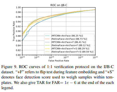
In Fig. 9, we show the ROC curves on the IJB-C dataset as well as the TAR for FAR= 1e − 6 at the end of each legend. We employ two tricks (i.e. flip test and face detection score to weigh samples within templates) to progressively improve the face verification accuracy. Under fair comparison, TAR (at FAR= 1e − 6) significantly improves from 88.29% to 89.59% simply by replacing MTCNN with RetinaFace. This indicates that (1) face detection and alignment significantly affect face recognition performance and (2) RetinaFace is a much stronger baseline that MTCNN for face recognition applications.
그림 9에서는 IJB-C 데이터 세트의 ROC 곡선과 각 범례의 끝에있는 FAR = 1e − 6에 대한 TAR을 보여줍니다.
얼굴 확인 정확도를 점진적으로 향상시키기 위해 두 가지 트릭 (예 : 플립 테스트 및 얼굴 감지 점수를 사용하여 템플릿 내 샘플 무게 측정)을 사용합니다.
공정한 비교에서 TAR (FAR = 1e-6에서)은 MTCNN을 RetinaFace로 대체함으로써 88.29 %에서 89.59 %로 크게 향상되었습니다.
이는 (1) 얼굴 감지 및 정렬이 얼굴 인식 성능에 상당한 영향을 미치고
(2) RetinaFace가 얼굴 인식 애플리케이션 용 MTCNN보다 훨씬 강력한 기준임을 나타냅니다.
4.8. Inference Efficiency 추론 효율성
During testing, RetinaFace performs face localisation in a single stage, which is flexible and efficient. Besides the above-explored heavy-weight model (ResNet-152, size of 262MB, and AP 91.8% on the WIDER FACE hard set), we also resort to a light-weight model (MobileNet-0.25 [22], size of 1MB, and AP 78.2% on the WIDER FACE hard set) to accelerate the inference.
테스트 중에 RetinaFace는 유연하고 효율적인 단일 단계에서 얼굴 위치 파악을 수행합니다.
추론을 가속화하기위해, 위에서 살펴본 헤비급 모델 (ResNet-152, 크기 262MB, WIDER FACE 하드 세트의 AP 91.8 %) 외에도 경량 모델 (MobileNet-0.25 [22], 크기 1MB, WIDER FACE 하드 세트의 AP 78.2 %을 사용합니다.
For the light-weight model, we can quickly reduce the data size by using a 7 × 7 convolution with stride=4 on the input image, tile dense anchors on P3, P4 and P5 as in [36], and remove deformable layers. In addition, the first two convolutional layers initialised by the ImageNet pre-trained model are fixed to achieve higher accuracy.
경량 모델의 경우 입력 이미지에서 stride = 4 인 7 × 7 컨볼루션을 사용하고 [36]에서와 같이 P3, P4 및 P5에 고밀도 앵커를 타일링하고 변형 가능한 레이어를 제거하여 데이터 크기를 빠르게 줄일 수 있습니다.
또한 ImageNet 사전 학습 된 모델에 의해 초기화 된 처음 두 개의 컨벌루션 레이어가 고정되어 더 높은 정확도를 달성합니다.
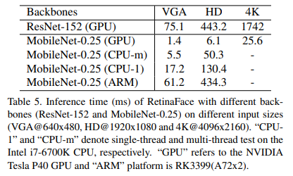
Tab. 5 gives the inference time of two models with respect to different input sizes. We omit the time cost on the dense regression branch, thus the time statistics are irrelevant to the face density of the input image. We take advantage of TVM [7] to accelerate the model inference and timing is performed on the NVIDIA Tesla P40 GPU, Intel i7- 6700K CPU and ARM-RK3399, respectively. RetinaFaceResNet-152 is designed for highly accurate face localisation, running at 13 FPS for VGA images (640 × 480). By contrast, RetinaFace-MobileNet-0.25 is designed for highly efficient face localisation which demonstrates considerable real-time speed of 40 FPS at GPU for 4K images (4096 × 2160), 20 FPS at multi-thread CPU for HD images (1920 × 1080), and 60 FPS at single-thread CPU for VGA images (640 × 480). Even more impressively, 16 FPS at ARM for VGA images (640 × 480) allows for a fast system on mobile devices.
Tab. 5는 서로 다른 입력 크기에 대한 두 모델의 추론 시간을 제공합니다.
조밀 회귀 분기(dense regression branch)에서 시간 비용을 생략하므로, 시간 통계는 입력 이미지의 얼굴 밀도와 관련이 없습니다.
모델 추론을 가속화하기 위해 TVM [7]을 활용하고 타이밍은 각각 NVIDIA Tesla P40 GPU, Intel i7-6700K CPU 및 ARM-RK3399에서 수행됩니다. RetinaFaceResNet-152는 VGA 이미지 (640 × 480)의 경우 13FPS에서 실행되는 매우 정확한 얼굴 위치 파악을 위해 설계되었습니다.
반면 RetinaFace-MobileNet-0.25는 4K 이미지 (4096 × 2160)의 경우 GPU에서 40FPS, HD 이미지 (1920 × 1080), VGA 이미지 (640 × 480)의 경우 단일 스레드 CPU에서 60FPS의 경우 멀티 스레드 CPU에서 20FPS의 상당한 실시간 속도를 보여주는 매우 효율적인 얼굴 위치 파악을 위해 설계되었습니다.
더욱 인상적인 것은 ARM에서 VGA 이미지 용 16FPS (640 × 480)를 통해 모바일 장치에서 빠른 시스템을 구현할 수 있습니다.
5. Conclusions
We studied the challenging problem of simultaneous dense localisation and alignment of faces of arbitrary scales in images and we proposed the first, to the best of our knowledge, one-stage solution (RetinaFace). Our solution outperforms state of the art methods in the current most challenging benchmarks for face detection. Furthermore, when RetinaFace is combined with state-of-the-art practices for face recognition it obviously improves the accuracy. The data and models have been provided publicly available to facilitate further research on the topic.
우리는 이미지에서 임의의 스케일의 얼굴을 동시에 조밀한 위치 파악 및 정렬이라는 도전적인 문제를 연구했으며, 우리가 아는 한 가장 먼저 1 단계 솔루션 (RetinaFace)을 제안했습니다.
당사의 솔루션은 현재 가장 까다로운 얼굴 인식 벤치 마크에서 최첨단 방법을 능가합니다.
또한 RetinaFace가 얼굴 인식을위한 최첨단 관행과 결합되면 분명히 정확도가 향상됩니다.
데이터와 모델은 주제에 대한 추가 연구를 용이하게하기 위해 공개적으로 제공되었습니다.
'지도학습 > 얼굴분석' 카테고리의 다른 글
| 3D Face Mesh Modeling from Range Images for 3D Face Recognition (0) | 2021.03.12 |
|---|---|
| Face Detection Ensemble with Methods Using Depth Information to Filter False Positives,2019 (0) | 2021.03.12 |
| Fast Facial Detection by Depth Map Analysis (0) | 2021.03.12 |
| MTCNN,2016 (0) | 2021.03.12 |
| 3D Face Mesh Modeling for 3D Face Recognition (0) | 2021.01.17 |


