Learning Facial Expressions with 3D Mesh Convolutional Neural Network
Making machines understand human expressions enables various useful applications in human-machine interaction. In this article, we present a novel facial expression recognition approach with 3D Mesh Convolutional Neural Networks (3DMCNN) and a visual analytics-guided 3DMCNN design and optimization scheme. From an RGBD camera, we first reconstruct a 3D face model of a subject with facial expressions and then compute the geometric properties of the surface. Instead of using regular Convolutional Neural Networks (CNNs) to learn intensities of the facial images, we convolve the geometric properties on the surface of the 3D model using 3DMCNN. We design a geodesic distance-based convolution method to overcome the difficulties raised from the irregular sampling of the face surface mesh. We further present interactive visual analytics for the purpose of designing and modifying the networks to analyze the learned features and cluster similar nodes in 3DMCNN. By removing low-activity nodes in the network, the performance of the network is greatly improved. We compare our method with the regular CNN-based method by interactively visualizing each layer of the networks and analyze the effectiveness of our method by studying representative cases. Testing on public datasets, our method achieves a higher recognition accuracy than traditional image-based CNN and other 3D CNNs. The proposed framework, including 3DMCNN and interactive visual analytics of the CNN, can be extended to other applications.
CCS Concepts: • Computing methodologies → Shape representations; Neural networks; Visual analytics;
Additional Key Words and Phrases: Facial expression analysis, 3D mesh convolutional neural networks, visual analysis
1 INTRODUCTION
Facial expressions play an important role in understanding human emotion status and have been widely studied since the 17th century [11]. Automatic facial expression recognition (AFER) requires interdisciplinary knowledge including behavioral science, machine learning, and artificial intelligence.
Exploring facial information through 2D images has been actively studied in the areas of emotion visualization [17], face recognition [41], age estimation [15], and facial expression recognition (FER) [2]. These techniques mainly rely on the features extracted from the 2D images and train statistic models to complete the classification tasks. The Active Appearance Model (AAM) [28], Active Shape Model (ASM) [1], and Constrained Local Model (CLM) [12] are three typical 2D-based methods for face tracking and recognition. Although these 2D methods have been proved effective in many constrained and unconstrained environments, their classification accuracy varies under different illuminations and orientations.
To avoid adverse effects caused by the external factors, one possible solution of the problem is to obtain more features directly from 3D space. Cohen et al. [9] proposed a 3D data-based facial expression recognition method for Human-Computer Interactions (HCI) using 3D laser scanners. Blanz et al. [5] presented a 3D face recognition approach based on Principal Component Analysis (PCA) decompositions of a 3D face database. Recent development of RGBD cameras has made 3D scanning easier, cheaper, and more accurate. A 3D object reconstruction method using an RGBD camera was presented by Newcombe et al. [31], which can be also used for face modeling. Chen et al. [8] showed a facial performance capturing method, and Thies et al. [40] presented a real-time expression transfer method for facial re-enactment. Since a depth camera provides 3D information in addition to the regular 2D images, it improves the accuracy of the detection and recognition and therefore enables more advanced applications.
The 3D information can also be provided to the 3D deep learning methods. Sinha et al. [37] presented a 3D model surface learning method based on CNN by creating a geometry image from the input 3D shapes. Su et al. [38] rendered 3D models to several 2D images using multiview methods and used them to train a Multiview CNN for shape learning. In a nutshell, these methods still transfer 3D shapes into 2D images as the input of the CNN framework. Instead of performing 2D operations in CNN, Wu et al. [43] used 3D voxel filters to process the voxelized depth data. Their model significantly outperformed existing approaches for shape recognition tasks.
To take advantage of the high-performance CNN and richer information in 3D-based methods, we propose a 3D Mesh Convolutional Neural Network, which performs general operations directly on the surface of the 3D mesh. In the facial expression recognition task case, these operations can be performed on the surface of the reconstructed 3D face model. To obtain a consistent sampling grid across the 3D faces, 3D face models are reconstructed by fitting a deformable face model to the scanned surfaces, in which a dense vertex correspondence can be roughly obtained. This property ensures that the processing operations including convolution and pooling are performed uniformly on the 3D surface.
More importantly, we propose a visual analytics approach to the learned features and networks, which is important for modification and optimization toward better performance of the network. Through an interactive visualization of the learned features and high-activation feature areas, our system can demonstrate clustered nodes based on their activation behaviors, which provides users intuitive visual analytics on the trained networks and allows them to interactively modify the networks. Based on the visualization result and through the interactions, users can better understand expected and discover unexpected features, network node performance, and so forth, and hence better fine-tune the trained network and optimize its performance as well as reduce the overfitting problems.
1.1 Related Work
Facial expression is the most direct reflection of emotion and shares common meanings across different races and cultures. Ekman and Friesen's (1975) study summarized six universal human facial expressions, including happiness, anger, sadness, fear, surprise, and disgust. These are also the most representative expressions for emotions and well utilized for emotion estimation and visualization purposes. A Facial Action Coding System (FACS) was proposed by Ekman and Friesen to describe facial expressions in a standard measurement. FACS is widely used in image-based facial expression recognition methods [13].
Extracting 2D features, such as displacement of feature points and intensity change from images, for facial expression recognition is the most popular method. Kobayashi et al. [23] presented an emotion classification method using 20 feature points on the face. Later studies, including ASM, AAM, and CLM, are also effective expression classification approaches based on 2D features. Kwang-Eun Ko et al. [22] presented a method using ASM to extract facial geometry features to estimate human emotions. Derived from ASM, AAM [10] both fits the facial image with geometric feature points and computes the intensities around the feature points. Lucey et al. [28] showed the capability of the AAM-based emotion estimation method using the Cohn-Kanade Dataset. Kapoor et al. [20] only used the pixel intensity difference to classify the expressions of human faces. One of the major limitations of these methods is that their estimation accuracy heavily depends on the image quality.
Even though 2D features are relatively easy to extract, they are not stable under various circumstances. Since the images are the rendered results under various extrinsic factors—lighting, camera location and angle, and so on—even the same object can be rendered significantly varyingly under different conditions. Sandbach et al. [33] presented that the illumination and the head pose were two significant factors affecting the recognition accuracy. Therefore, in order to alleviate the influence of these factors, 3D geometric features, like curvature, volume, displacement, conformal factor, heat kernel signature, and shape spectrum, were often used in recent 3D-based approaches. Since the 3D features are pose and illumination invariant, they are more stable and consistent than the 2D features in different circumstances. Huang et al. [35] extracted the Bézier volume change as the features of the emotions, and Fanelli et al. [14] used the depth information of pixels to classify emotions. These studies successfully embedded 3D features in the facial expression recognition task and demonstrated their effectiveness. Therefore, to extract accurate 3D geometric features, high-quality 3D face capturing with arbitrary facial expressions is essential.
Recently, there have been several remarkable achievements in 3D face reconstruction. Lei et al. [25] presented a face shape recovery method using a single reference 3D face model. Prior knowledge of face is required for these methods to recover the missing depth information from a 2D image. Learning through a face database is another effective approach for tackling this problem. Along this direction, statistical face models based on PCA were proposed and constructed [4]. As these approaches achieved plausible 3D face reconstruction results based on 2D images, Blanz et al. [5] applied the 3D face reconstruction method to the facial recognition problem. However, these methods are still limited to the neutral expression and produce poor reconstruction results on faces with expressions. Therefore, incorporating the RGBD camera with a deformable 3D face model can provide a fast and accurate 3D face model for geometric feature extraction.
In terms of the classification models, the traditional facial expression classification method mainly uses texture features, such as Haar [42] and Local Binary Pattern (LBP) [48], to train a statistical classifier such as Linear Discriminant Analysis (LDA) [3], PCA [44], and Support Vector Machine (SVM) [36]. With the recent development of high-performance deep learning techniques, such as Convolutional Neural Networks (CNNs), image recognition accuracy has been greatly improved [24, 34]. Applying CNNs to the facial expression recognition problem, Kim et al. [21] employed multiple CNNs to obtain a group of diverse models with various properties. Mollahosseini et al. [30] trained a single CNN based on multiple naturalistic datasets to obtain a high-performance model across datasets. Zhang et al. [47] presented a method for inferring social relations from face images using CNNs. They presented a pairwise-face reasoning for relation prediction based on the subjects’ age, gender, expression, and head pose. Lopes et al. [27] proposed a method that combines CNNs and preprocessing techniques to reduce the data required for CNN training.
To extend the high-performance CNN framework to the 3D model classification task, Sinha et al. [37] proposed a 3D shape learning method using geometric images. Su et al. [38] used a multiview rendering method to render a 3D shape to a number of rendered image series from different angles. Multiview image-based CNN may work well on 3D models with large variations in different views as shown in [38]. However, in the classification of facial expressions, views from significantly different angles do not provide extra expressional information as most features are often distributed on the frontal surface. Wu et al. [43] worked on the volumetric shapes for deep learning. To simplify the deep learning framework, these methods transfer 3D shape to a uniform square domain or cubic domain instead of computing directly on the shape surface. This is a straightforward solution for 3D shape classification with CNNs, especially learning various different shapes. However, the 3D shapes in the facial expression recognition task are all 3D facial models, which provide the possibility of normalizing them to a standard facial area domain. Utilizing this property, we propose a 3D Mesh Convolutional Neural Network for facial expressions on the 3D facial surfaces.
To better understand the learned features of the network, Zeiler et al. [46] proposed a CNN visualization method for diagnostic purposes, and Liu et al. [26] presented a directed acyclic graph-based CNN visualization method to obtain an overview of the CNNs. More recently, Pezzotti et al. [32] presented a progressive visual analytics approach for designing CNNs and successfully optimized the public large-scale CNNs using the insights obtained from their system. Kahng et al. [19] presented a method to visually explore industry-scale Deep Neural Networks. Inspired by these CNN visualization methods, we develop a 3D Mesh CNN visualization framework, which focuses on the learned 3D features and network optimization as well as their relations.
In this article, we present a novel robust approach for facial expression recognition based on 3DMCNN that learns 3D features of the reconstructed face models. We use a 3D facial expression database to fit the scanned depth image of the face to generate a high-quality 3D face model with expressions. Then, we compute the geometry signatures, i.e., mean curvature, conformal, factor, and heat kernel signature, as the features for learning. We perform the learning processes, such as convolution, pooling, rectified linear unit (ReLU), and so forth, directly on the 3D surface domain for training the 3DMCNN. Through visual analytics, we can modify and optimize the networks for better performance. Finally, we compare the performance of our method with conventional image-based CNN methods and analyze the advantages of our method by using interactive visualization techniques. Figure 1 illustrates the entire process.

Fig. 1. The pipeline of our 3D face model-based facial expression recognition framework with 3D Mesh Convlutional Neural Networks. Based on the captured depth image and facial landmarks on the color image, a 3D facial expression model is generated by fitting a morphable face model. The geometric signatures of the 3D facial model are computed and used for training a 3DMCNN for classifying facial expressions.
Our contributions in this article are summarized as follows:
- We propose a 3D Mesh Convolutional Neural Network for learning facial expressions on 3D face models. Our method convolves 3D signatures directly over an irregular sampled surface based on the geodesic distance.
- We present a visual analytics framework for deeper understanding of the automatic feature selection and node activation procedure, and provide interactive node selection and removal operations for network modification and optimization.
- Our method is robust on the rotation of the face and environmental illumination variance since it focuses on the surface geometry descriptors as learning features instead of the intensities of the regular images.
The rest of the article is organized as follows: Section 2 introduces the method for reconstructing the 3D face with expressions using the RGBD camera and deformable face model. In Section 3, we explain our 3DMCNN and its geodesic distance-based convolution and pooling framework. Then, the employed geometric descriptors of the 3D face are described. Section 4 introduces the learned feature maps and the clusters of different nodes in our 3DMCNN, which facilitates further editing of the networks based on an interactive visual analytics approach. In Section 5, we first show the public database for the experiment and then explain the training and testing details. Finally, we show the results of our method and compare it to state-of-the-art 2D image-based CNN methods and other CNN methods for 3D shapes.
2 3D FACE RECONSTRUCTION FROM RGBD SENSOR
We employ a Kinect v2 system that captures 1920x1080 2D images and 512x424 depth maps at 30 frames per second. A raw depth image of the subject's face along with RGB color information is acquired. To improve the quality of the raw 3D facial data and normalize it to a uniform face data space, we use a multidimensional 3D face database, Facewarehouse, as a refinement template. Cao et al. [7] presented a 3D facial expression database, which includes 150 subjects with 47 different expressions. The database is decomposed in a bilinear face model and each face model can be computed by
S=C×2wiT×3weT,(1)
where C is the decomposed core tensor, wi is the identity weight vector, and we is the expression weight vector, respectively. Then, the identity weight wi and the expression weight we can be obtained by minimizing the surface distance between the scanned raw face S^ and the reconstructed bilinear model S as follows:
wi,we=argmin‖S^−(R(S)+T)‖2,(2)
where R is the rotation matrix and T is the translation matrix. In practice, we first estimate the rotation angle and translation using the method [ 18], and then we optimize identity weight wi, followed by optimizing expression weight we. To fine-tune the expression of the generated 3D face model, we utilize the RGB color image that is captured simultaneously with the depth map. We use the Constrained Local Model (CLM) [ 12] to find 74 landmarks on the color image. These points include the face contour, eye contour, and eyebrow, nose, and mouth contour, which are used for the following two purposes. One is that these landmark points can be used for locating the face position in the image and estimating the head rotations. Estimating head rotation is important to initialize the template face model to start the fitting process. The second is that the points can be used to fine-tune the reconstructed expressions to improve the reconstruction accuracy of certain extreme expressions. The left block in Figure 1 illustrates the reconstruction process.
There are two advantages of using the face decomposition approach to reconstruct the 3D faces. First, it provides an easy and low-cost solution to obtain higher-resolution 3D face models for expression analysis. Traditional high-resolution 3D scanners are expensive, and the scanning usually takes a long time. Therefore, capturing a facial expression is a difficult task for this equipment. Meanwhile, although the commercial depth camera can provide a cheap and fast way to scan faces, the reconstructed 3D meshes often have low resolution for computing meaningful geometric features for learning facial expressions. The face decomposition approach can use a prescanned database as a prior knowledge to generate 3D high-resolution facial expression models from low-resolution depth scans. Second, it provides a consistent sampling domain across the generated 3D faces. Since the optimized 3D face model is obtained by computing the weight vectors, it is actually a linear combination of the decomposed basis faces. The generated 3D face always has one-to-one correspondence in terms of vertex to the average 3D face of the database S¯. Therefore, the sampling points on the 3D faces across the subject and the expressions are consistent. We use the consistent sampling points as the grids to perform CNN computations, which will be explained in detail in Section 3.
3 3D MESH CONVOLUTIONAL NEURAL NETWORKS
In this section, we present a 3D Mesh Convolutional Neural Network (3DMCNN) for facial expression recognition by learning facial geometric features. Our method conducts operations including convolution and pooling by utilizing the mesh grid on a template face model as shown in Figure 2(a). The red points are the sampling grid for computation, equivalent to the pixels in 2D CNN. Instead of using a regular uniform grid in 2D image CNN, we have denser grids around high-activity and -curvature regions including the eyes, mouth, and wrinkles near the mouth for a higher sampling rate.

Fig. 2. (a) Illustrates the sampling points on the face surface. (b) Illustrates the continuous geodesic distance rings around the center points. (c) Illustrates the discrete eight directions for geodesic distance-based convolution. (d) Shows the normal vector of the sample point for tangent plane computation and the defined directions.
3.1 Geodesic Distance-Based Convolution and Pooling
Convolution: Traditional CNN uses a uniform grid for convolution and pooling, which is efficient for processing images. Instead of transforming 3D surfaces to 2D planes for learning, our method directly learns the geometric features on the 3D surface. Since the reconstructed 3D face is a linear combination of the decomposed basis faces, there is one-to-one correspondence in terms of vertices across the face models by nature. These vertices serve as the consistent sampling points on the face domain for CNN computation, which is shown in Figure 2(a). The red points are sampling points on the face surface and we compute the convolution on each point.
Similar to the convolution on an image, we use a weighted filter to convolve the geometric signature values. Convolution on images is done by sliding a square filter over the images; however, defining a square filter on the 3D surface is difficult. To solve this problem, we propose a geodesic distance-based convolution, where the weights are defined by the geodesic distances. In a continuous form of geodesic distance-based convolution, the weight values are continuous functions to the geodesic distance from the center point. To reduce the computational cost on the discrete meshes, we define limited directions for convolution. On each vertex, we search eight directions, which are east, northeast, north, northwest, west, southwest, south, and southeast, as shown in Figure 2(b). Together with the center point, we denote these directions as D, which is illustrated in Figure 2(c). We define the east direction as the x→-axis increasing direction and similarly define the north direction as the y→-axis increasing direction based on a standard world coordinate system. Newly reconstructed 3D face models are first scaled and rotated to the front-facing position (i.e., the standard coordinate system), so that the directions can be consistently defined across all the models. To search for the east direction, we start from the center point and search over the surface until it reaches the defined geodesic distance. The normal vector of the center vertex is needed to compute the tangent plane, and the initial searching directions are defined on the tangent plane. Similarly, we search for the other seven directions and compute the weighted sum around the center point as follows:
gn+1=∑d∈D(w(d,l)g(d,l)n),(3)
where w(d,l) is the weights defined by the distance l and direction d, g(d,l)n is the geometric signature value at the destination location, and n indicates the layer of the network. As the geometric signature values are only defined at the sampling points, it is not guaranteed that we can find a value at the destination location. By using the barycentric interpolation of the nearby triangle, we can compute the value g(g,l)n at any location of the surface.
The geodesic distance-based convolution has the advantages of preserving and identifying true features as well as preventing dislocated false features in the convolution space when taking the actual geodesic distance as a priori information. Figure 3 shows an illustrative one-dimensional example, where the curve is the shape and the line segment indicates the pixels of the 1D “image” of the curve shape. The sampling vertices V1, V2, V3, and V4 on the curve are rendered to the pixels P1, P3, and P4 on the 1D “image.” As shown in figure, although V2 has a high curvature value on the curve, it is not rendered on the “image” due to the sampling interval. When the convolution is done on the image plane without considering the geodesic distance, a low curvature value at V3 will be used for convolution instead of V2’s curvature value. Therefore, the important geometric feature of vertex P2 will be lost in the image convolution framework, which is not desired. On the other hand, the image convolution framework will result in an uneven convolution on the 3D surface domain. For example, the surface patches that are perpendicular to the image plane will be coarsely sampled and the parallel surface will be densely sampled. So using geodesic distance for convolution avoids these problems caused by simply applying the image convolution framework to the 3D surfaces and provides more uniform convolution results. This is also evidenced by our later experiments in Section 5.

Fig. 3. Illustration of the difference of pixel-based convolution and the geodesic distance-based convolution. Color shows two rendered pixels P1 and P2 from the mesh patch around vertex V1 and V3. V2 is not rendered individually due to the resolution.
Pooling: Similar to the convolution, we also perform a pooling operation based on geodesic distance. Based on the selected geodesic distance, we compute the mean (or max) value of the feature values over a region within a certain geodesic distance around the sampling point. Since the sampling points become sparse after each pooling operation, we retriangulate the remaining sampling points to reconstruct a new mesh surface and double the geodesic unit for the next layer computation. Once the 3DMCNN architecture is established, the resampling of the 3D faces can be precomputed before the training process. We generate a cascaded face series with the reference face and map to each individual model. The geodesic unit is determined by the average geodesic distance between two sampling points on the shape surface. As we mentioned above, we increase the geodesic unit based on the stride of the pooling operation.
3.2 Architecture of 3D Mesh Convolutional Neural Networks
The layers of the 3DMCNN are determined by the complexity of the 3D models and the size of the database. Our 3D face model approximately consists of 5,000 vertices and has about 60 × 80 sampling points on the surface. For each expression, there are 800 models with different identities. Therefore, we only need a relatively shallow architecture for the networks. Our CNN model has three convolution (C1, C2, C3) and pooling layers (P1, P2, P3) and two fully connected layers (FC1, FC2). Specifically, C1 is a convolutional layer with feature maps connected to a neighboring area within the 2 geodesic units in the input.
The values in C1 are initialized by a uniform distribution with the range depending on the incoming nodes. P1 is a pooling layer with feature maps connected to corresponding feature maps in C1. In our case, we use the max pooling to amplify the most responsive vertex in the feature maps. C3 uses a partial connection scheme for keeping the number of connections within proper bounds and breaking symmetry in the network. In this way, we can expect the kernels to update diversely to generate different feature maps.
3.3 3D Descriptors for Deep Learning
In this section, we discuss the 3D descriptors that are used for the mesh CNN training. Generally, 3D properties including principal curvatures, mean curvatures, Gaussian curvatures, conformal factors [16], and heat kernels [39], can be used to describe the 3D shapes. As Hua et al. [16] indicated that a 3D shape can be uniquely defined if the mean curvatures and the conformal factors are given, in this article, we use mean curvature, conformal factor, and heat kernel as the geometric descriptors of the 3D face model. These features are normalized to the range between 0 and 1 before training.
3.3.1 Mean Curvature. Mean curvature measures the average curvature at a given point of a surface S, and it is also equal to the average of the principal curvatures. On a discrete triangular mesh, we compute the mean curvature at point p by
H(p)=14A‖∑q∈N(p)(cotα+cotβ)pq→‖2,(4)
where α and β are two opposite angles of the shared edge pq→ in two triangles, and N(p) is the set of 1-ring neighbor vertices of vertex p. A is the Voronoi area of the vertex p, which can be computed by
A(p)=18∑q∈N(p)(cotα+cotβ)‖pq→‖2(5)
if the triangles in the 1-ring neighborhood are nonobtuse. Meyer et al. [ 29] presented the solution for the obtuse case. Figure 4 illustrates the angles and the area of the vertex p.

Fig. 4. α and β are the opposite angles to the edge pq→. Yellow area shows the Voronoi area associated to the vertex p.
Figure 5 shows the mean curvature on 3D meshes of three examples: an armadillo, a human brain, and a scanned human face. The mean curvature values are normalized to the range from 0 to 1 and mapped to RGB colors for visualization. Regions such as fingertips, brain sulci, eye contour, and mouth show red, which have high curvatures. Mean curvature provides the face mesh deformation information for learning the expressions. Mean curvature is a local property that can be computed at each vertex in discrete mesh forms; therefore, the computation can be easily parallelized using GPU.

Fig. 5. Illustration of mean curvature on three different shapes. The mean curvature values are normalized to [0, 1], and the color map is shown on the right.
3.3.2 Conformal Factor. Conformal factor measures the vertex area change of the deformed shape. The discrete conformal factor can be defined as
λ(p)=Ae(p)An(p),(6)
where the Ae(p) and An(p) are the averaging areas of the vertex p on surface e→ and n→.
The conformal factor function λ(u,v) and the mean curvature function H(u,v), defined on D, satisfy the Gauss and Codazzi equation, as a conformal surface S(u,v) is parameterized on a domain D. Therefore, if λ(u,v) and H(u,v) are given with boundary conditions, the surface S(u,v) can be reconstructed uniquely. The mean curvature and the conformal factor are two important signatures that carry fundamental information of a surface. These two signatures can be used for training 3DMCNN. In our case, e→ is the surface of the 3D face with an expression and n→ is the surface of the 3D face with a neutral expression, which can be obtained once the identity weight vector wi is estimated.
Figure 6 shows an example of the conformal factors on the 3D facial model. Figure 6(a) is a nonneutral expression. Figure 6(b) is a neutral expression face, which is reconstructed once the identity vector Wi is estimated. Based on the computed Voronoi area using Equation (5), the conformal factor λ(p) is computed based on least square conformal mapping. The conformal factors are normalized and visualized with color map as shown in Figure 6(c). The highlighted areas in Figure 6(c) show the significant changes around the mouth, where the main deformations occurred.

Fig. 6. Illustration of the conformal factor on a facial expression model. (a) Nonneutral facial expression model. (b) Estimated neutral expression model after the identity vector Wi is obtained. (c) Conformal factor map. The two highlighted areas show the area change of the surface.
3.3.3 Heat Kernel Signature. A heat kernel signature (HKS) is a feature descriptor of a spectral property of a 3D shape and is widely used in deformable shape analysis [39]. HKS defines local and global geometric properties of each vertex in the shape by a feature vector, which is used for segmentation, classification, structure discovery, shape matching, and shape retrieval. The HKS k is a function of time t, which can be solved by the differential equation δhδt=−Δh. The HKS at a point p is the amount of remaining heat after time T, which is
k(p)=∑i=0∞e−TλiΦi2(p),(7)
where λi and Φi are the ith eigenvalue and eigenfunction of the Laplacian-Beltrami operator. The HKS is an intrinsic property of a given mesh; thus, it is stable to noises and articular transformations or even some topological changes. The HKS is also a multiscale signature of the shape, which means changing the time parameter T can control the scale of the signature. For example, a larger T represents a more global feature and a smaller T represents a more local feature of the shape. Figure 7 illustrates the heat kernel signatures of two expressions. The time variable T increases from left to right, showing the continued change of HKS on the face surfaces. Since HKS is a global feature of the shapes, it is widely used for shape analysis and shape retrieval tasks due to its significant differences between different shapes [ 6]. Although the HKS is relatively stable on the human face models, we found it also changes with the different expressions, especially with the smaller time parameters. To use more significant local differences as the feature while keeping a certain level of the global feature, we experimentally select a small T = 10 in our method. Therefore, HKS performs as a supportive feature to the more sensitive mean curvature and conformal factor in the 3DMCNN framework.

Fig. 7. Heat kernel signature on two different facial expression models. Left to right shows T = 10, 20, 30, 40. Upper row shows a sample face with surprised expression and the lower row shows a sample face with neutral expression.
4 VISUAL ANALYTICS OF NETWORKS FOR MODIFICATION AND OPTIMIZATION
In this section, we present an interactive visual analytics method of the 3DMCNN for the purpose of network performance. First, to better understand the 3DMCNN, visualizing the learned features of neurons is an effective approach. Liu et al. [26] presented a directed acyclic graph-based CNN visualization method, which explores features and network structures by clustering similar neurons and visualizing them in a properly ordered layout. Their method focuses on visualization of the deep CNNs without interactive modification of the network.
Inspired by their method, we present an interactive neuron visualization and modification framework, which provides intuitive and detailed information for understanding and optimizing the network. Our visualization framework enables three abilities: first, find salient features of geometric signatures that affect the expression recognition result; second, find expression-specific features for each expression; third, modify the networks by removing unnecessary neurons with low activation values for network simplification. As we cannot accurately know how many neurons and layers are needed for training the 3DMCNN at the beginning, we usually provide a sufficient number of neurons and layers as an initial setup. Then, the neurons with high activations for certain expressions are clustered and the layouts of the network are rearranged accordingly. By analyzing these different clusters of neurons, we can understand important features and the neurons that are sensitive to them. By selecting the significant features and high-activation neurons as the initial state of the retraining, the network structure can be simplified and the performance can be optimized.
Figure 8 shows an example for the visual analytics interface of the trained 3DMCNN. The network shows the first two layers, and each layer is composed by a convolution layer, a Rectified Linear Unit (ReLU) layer, and a pooling layer. A three-channel input data is passed to the 3DMCNN, and we visualize the first two groups of layers. One of the neurons in the second layer is selected, the corresponding feature map is shown, and the connected neurons in the first layer are highlighted. For the connections between neurons, the associated filters are displayed as well. The interactive inspection approach enables us to find and analyze the important features.

Fig. 8. Illustration of the network visualization approach. The selected neuron in layer 2 is highlighted in yellow and its feature map is shown. The connection with the neurons in layer 1 is shown and the associated filters are displayed accordingly.
Clustering similar neurons into several functioning groups provides a clear overview of the learned network. In our visual analytics framework, the neurons are clustered into three types of groups: (1) high-activation positive nodes, whose associated weights are large positive values—these nodes contribute positive features to the output nodes in the next layer; (2) high-activation negative nodes, whose weights are large negative values; (3) low-activation nodes, whose associated weights are approximately zero. These nodes provide almost no features to the output layers, so they have no potentials and can be removed to reduce the network complexity and improve the performance of the network.
As illustrated in Figure 9, a set of smiling 3D face data is passed to the trained 3DMCNN. The nodes in each layer are clustered and visualized, and the associated spectrum colors represent the different activation values. High-activation positive nodes are labeled in red, low-activation nodes are labeled in green, and high-activation negative nodes are labeled in blue. We treat a node as a low-activation node if the total contribution to the final output is less than 5%. The connectivities are also grouped for simplified visualization of the network. In Figure 9, we trace back the classification result, for example, “happiness,” to explore the learned feature patches. We consecutively select the high-activation positive nodes to see the lower-level neurons connected to them. Shallow layers of the CNN detect detailed features such as contours and color patches, while deeper layers detect more global features such as detecting the parts of the objects. As we learned by visualizing the feature maps in each layer, our 3DMCNN also learns the expressions in a similar manner: it detects feature patches and then detects larger areas of the face and their combinations. Since we start training the network with a sufficient number of neurons, there exists many redundant neurons. Visualizing and interactively removing these redundant neurons improve the network efficiency, simplify the network, and reduce the overfitting problems.
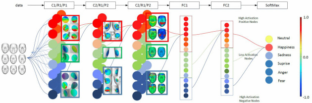
Fig. 9. Illustration of the feature visualization process. Red cluster contains high-activation positive nodes, green cluster contains low-activation nodes, and blue cluster contains high-activation negative nodes. Gray nodes are unconnected nodes to the selected node. Sample feature maps are displayed beside each cluster.
5 EXPERIMENT
We have applied our algorithm on public 3D face expression databases and Kinect scanned face models. The surface geometric features are experimented on first, followed by the training setups for the 3D MCNN. We compare our method with the 2D CNN-based method and geometry image-based method for facial expression recognition. Then, we analyze cases in which our method performs better than other methods. Our experiments have been performed on a Linux PC with 3.0GHz eight-core CPU, 8GB memory, and GeForce 980 graphics card with the NVIDIA CUDA Framework 6.5. The computation time of our method is mainly spent on the 3D Mesh CNN training process. The reconstruction and feature computation time for 3D face is approximately 3 seconds for each image.
5.1 Datasets
To evaluate our method, we employ two public 3D expression databases for training and testing. FaceWarehouse is used for training and 3D face generation in the testing phase. BU-3DFE is used for testing and comparison among different learning methods.
FaceWarehouse [7]: FaceWarehouse is a database of 3D facial expressions for visual computing applications. It includes 3D face scans of 150 individuals aged between 7 and 80 from various ethnic backgrounds. There are 20 expressions including neutral expressions for each person. For each expression, both the 3D model and the 2D image with landmarks are provided. The landmarks include important facial feature points, which can be used for fine-tuning the reconstructed 3D faces. The 3D face models with expressions are obtained by deforming a template facial mesh to match the scanned depth image. These meshes with consistent topology are assembled as a rank-3 tensor to build a bilinear face model with identity and expression. In our experiment, the expressions are manually labeled for six prototypic expressions (happiness, disgust, fear, angry, surprise, and sadness).
BU-3DFE (Binghamton University 3D Facial Expression) Database [45]: The BU-3DFE database includes 100 subjects (56% female, 44% male), aged from 18 to 70, with a variety of ethnic backgrounds, including white, black, East Asian, Middle East Asian, Indian, and Hispanic Latino. There are seven expressions for each subject including neutral expressions and the six prototypic expressions. For each nonneutral expression, there are four 3D shapes with four levels of intensity. Therefore, there are 25 instances of 3D expression models for each subject, resulting in a total of 2,500 3D facial expression models in the database. A color facial image is associated with each expression shape model.
5.2 Visual Analytics-Guided CNN Design and Optimization
We train the 3DMCNN with the FaceWarehouse dataset and test with the BU-3DFE dataset. Since there are symmetric and similar expressions, the data is manually labeled in five nonneutral classes and one neutral class. To improve the training robustness, we generate some randomness (±5%) to the 3D face reconstruction process to obtain more training datasets: (1) Add a random variance to the identity coefficient wi to generate a new identity. (2) Add a random variance to the expression coefficient we. Including the original 150 faces of the subjects and 450 synthetic data, we prepare 600 faces for each expression. We compute the three types of signatures on the 3D faces. Figure 11 illustrates the computed geometry signatures: (a) mean curvature, (b) conformal factor, and (c) heat kernel. The geometry features show similarity within the same expression across different subjects while varying between different expressions.
We start with three layers of the convolution layer, ReLU layer, and pooling layer, followed by two fully connected layers and a SoftMax classification layer. We set the number of nodes to 192 for convolution layer 1, and 256 for both convolution layers 2 and 3, respectively, which we consider as sufficient numbers for neurons. We set the weight update ratio to 0.0005 and run for 20,000 iterations. Once we obtain the initial classification network, we use our node clustering and visualization method to selectively remove low-activation neurons and retrain the network with the selected high-activation neurons as the initial status. An example of the optimization process is discussed in the following section. Figure 10 shows the evaluation results of the network simplification sessions. After 20 sessions of modification of the network based on our visual analytics approach, the training time, the number of nodes, and the number of maximum iterations are reduced while keeping a similar prediction accuracy. The final nodes are set to 128 for convolution layer 1, 192 for layer 2, and 256 for layer 3. Using the final network, we test on the public database and the results are discussed in Section 5.4.

Fig. 10. Evaluation of the interactive network simplification. Graphs show the training time, accuracy, node number, and maximum iteration with respect to the modification sessions.

Fig. 11. The geometry signatures on the 3D face. Each row shows different expressions of the same subject. Expressions 1, 2, 3 show three expressions: happiness, anger, and surprise. In each expression, column (a) shows the mean curvature, column (b) shows the conformal factor, and column (c) shows the heat kernel signature.
5.3 Case Study
In this section, we provide further details on the analysis performed with our visual analytics approach. As we discussed in Section 5.2, we optimize the network by reducing the redundancy. Since we start with a sufficient number of neurons, it usually generates many low-activation neurons, which increases the computational cost without contributing to the classification result. These neurons often have low connectivity to the subsequent layers as well. Our goal is to reduce the number of neurons with low activation values and low connectivity. We use the histogram plots to observe the distributions of the activation values. Figure 12 shows the activation histograms of the convolutional layers. Activation values were scaled to a range between −1 and 1, and 21 bins were selected to generate the histograms. Typical feature maps of the clusters are displayed accordingly on the histograms. The detailed lists of the neurons can be shown by selecting the histogram bins. The upper row of Figure 12 shows the initial stage before the network tuning, and the lower row shows the final stage after optimization. Initially, there is a large number of low-activation nodes in convolution layer 1 as shown in the histogram. We further inspect the learned features via the filter list. Figure 13 shows the list of the selected cluster of the neurons in an increasing order of the activation value. The connectivity (out) shows how many neurons in the subsequent layer are connected and the connectivity (in) shows how many preceding neurons are connected. The list can be rearranged by selecting different orders. We remove those neurons with low activation and connectivity and then retrain the network by keeping the rest of the feature maps. The neuron selection and removal can be reversed if the result shows unexpected changes. The bottom row of Figure 12 shows the activation histograms in the final stage, where the number of the low-activation neurons were greatly reduced compared to other neurons. Based on the modification using our visual analytics approach, we optimize the network by reducing the first convolutional layer from 192 to 128 filters, and the second convolutional layer from 256 to 192. The optimized result provides a compact network with reduced training time and the similar prediction accuracy.

Fig. 12. The activation histograms of the convolution layers. The upper row shows the histograms of the initial stage and the lower row shows histograms of the final optimized stage. Some sample filters are displayed on the histograms.

Fig. 13. The detailed inspection on the selected group of neurons. The table shows the list of the filters with low activations.
5.4 Comparisons and Evaluation
We evaluate our 3DMCNN framework by selecting different geometric signatures separately as well as their combinations to train a 3DMCNN. To fairly compare their performance in terms of providing sufficient features for training, we use the same 3DMCNN architecture and the same number of training data. Table 1 shows the test accuracy for each expression as well as the average. Mean curvature achieves the highest accuracy for 3DMCNN using the single feature only, followed by the conformal factor, while heat kernel achieves the lowest accuracy. This is because mean curvature and conformal factor carry more detailed information than heat kernel in local areas. Combining the three signatures as three channels of the input significantly improved the classification accuracy.
Table 1. Training Accuracy Based on Single Geometry Signature and Their Combination for Each Expression
FeaturesNeutral (%)Happiness (%)Sadness (%)Angry (%)Surprise (%)Fear (%)Average (%)
|
Mean Curvature |
85.2 |
83.5 |
82.3 |
85.6 |
83.1 |
83.3 |
83.8 |
|
Conformal Factor |
80.1 |
82.6 |
80.2 |
75.1 |
77.5 |
78.5 |
79.0 |
|
Heat Kernel Signature |
60.1 |
56.2 |
62.1 |
66.7 |
51.6 |
53.6 |
58.4 |
|
Combined |
92.3 |
90.1 |
89.5 |
88.1 |
90.2 |
89.6 |
89.8 |
We also compare our method with several existing methods: (1) traditional image-based CNNs [27], which uses images to train the CNNs; (2) geometry image CNNs [37], which map the 3D shape to the 2D image and generates synthetic geometric images for training regular CNNs; and (3) volumetric CNNs [43], which extend 2D image CNNs to 3D cubic CNNs. These methods are proposed for general 3D shape recognition purposes, and we employ them to our face expression recognition application for comparisons. We also implement an extra two types of methods derived from our method. (4) The 3D faces with their geometric signatures are rendered to projection images with virtual cameras and take the images for training and testing. We denote this method as the projection image-based method. (5) Since we capture the RGB information with the depth value simultaneously, we are actually able to obtain 3D faces with RGB textures. We combine this color information with geometric signatures to train a six-channel 3DMCNN, denoted as 3D Mesh&Image CNN. We compare these methods under the same configuration of the network architecture, i.e., same number of layers and neurons. Figure 14 summarizes the results. Our 3DMCNN and 3D Mesh&Image CNNs achieved the highest accuracy. Geometric image CNNs [37] also achieve a high classification accuracy (85%), since they also focus on the geometric features. However, the 2D authelic mapping used in the method does not guarantee a distance-preserving mapping, since the convolution on the 3D surface domain is nonuniform. The projection image-based method achieves slightly higher accuracy than the RGB image-based method, but lower than our mesh-based method. This is because they both learn other face-related features, such as face contour, color patch, and so on. Volumetric CNNs achieve the lowest accuracy, since they need extra depth of the network to reach their best performance. As a result, our method achieves the best accuracy (90%) under a shallow and compact network configuration.

Fig. 14. The comparison result between our method and other CNN-based methods. Our method achieves the highest recognition accuracy.
5.5 Knowledge from Visual Analytics of CNNs
Our visualization system provides an interactive way of neuron cluster selection for visualizing the learned features. By selecting the highest-activation cluster, the features are deconvolved back to the input 3D face space and the areas are highlighted. These areas are important since they lead to the strongest responses in the CNNs. Figure 15 shows the high-activation areas for two different expressions. The top nine high-activation areas are selected for demonstration in each expression. Figure 15(a) shows the features of the “happiness” class and Figure 15(b) shows features of the “anger” class. High-activation areas for happiness are mostly located around mouth corners as shown in the result. Furthermore, these features have strong reaction on mean curvature and only one feature area reacts on the conformal factor (lower left of Figure 15(a)). On the other hand, high-activation areas for “anger” are distributed around the eyes and forehead. In contrast to the “happiness” class, four areas react to conformal factors for the “anger” class. From the visualization result, we know different geometric signatures carry different information for certain expressions. Figure 16 shows the high-activation areas for “happiness” and “anger” for comparison. We map these areas to the template face domain for consistent visualization purposes. Features are located around the mouth and eyes for “happiness.” Since features around the eyes are also considered as important as mouth corners, the 2D image-based method may not work well for some ambiguous expressions. Figure 17 shows three examples where the image-based method fails to correctly classify the expressions; however, we successfully classify it using our method. Figure 17(a) shows that the subject unintentionally closed her eyes while smiling, which leads to misclassification in the 2D image-based method. Figure 17(b) shows the case is classified to “anger” using the image-based method under extreme illumination, whereas it was classified to “happiness” using our method. Figure 17(c) shows the failed case for the image-based method under large rotation. Our method provides a robust and stable classification outcome to some ambiguous expressions and also under some uncontrolled environment conditions and extreme head poses.

Fig. 15. High activation feature areas on 3D face surface of two expression classes: (a) is happiness and (b) is anger. All the feature areas are mapped to the template face for consistent visualization.

Fig. 16. High-activation feature areas on 2D images of two expression classes: (a) is happiness and (b) is anger.

Fig. 17. Successful classification cases using our method while the 2D image-based method misclassified.
5.6 Limitations
Although the proposed 3D mesh CNN can achieve high performance on facial expression recognitions, there are two main limitations. One is that our method needs a uniform sampling standard across the 3D shapes. This is because, similar to the image-based CNNs, the computations of convolution and pooling need to be performed consistently on the 3D surface under a uniformly defined structure. Further studies need to be done to apply the 3DMCNN to general classification tasks. The second limitation is that the 3D deformable face model contains limited high-frequency details. Fine local details such as wrinkles are not properly modeled and therefore result in the fitted model not containing this information either. Therefore, some subtle expressions with tiny facial deformations cannot be predicted accurately using current 3D face models and data. This disadvantage would affect the potential peak performance of the 3DMCNN to learn deeper features using a smaller size of convolution filters.
6 CONCLUSION
In this article, we have presented a 3D Mesh Convolutional Neural Network for facial expression recognition and an interactive visual analytics method for the purpose of designing and modifying the networks. Based on the depth surface scanning via an RGBD camera, we have reconstructed a 3D face model by fitting a deformable face model to the raw surface. We have adopted three types of geometric signatures, including mean curvature, conformal factor, and heat kernel, as feature values of the shape surface. These signatures can comprehensively describe the shape surface both locally and globally. Using the geometric signatures, the 3DMCNN is trained. To uniformly convolve the sampling points on the face surface, we proposed a geodesic distance-based convolution scheme. This geodesic distance-based convolution and pooling method can prevent dislocated false features and preserve actual local features. We have trained and tested the 3DMCNN using two public 3D face expression databases and analyzed the effectiveness of our method by interactively visualizing the learned features on the neurons. Through the visualization results, we have demonstrated some high-activation features that affect the recognition result most. We have compared our method with the traditional image-based CNNs, and our method achieves higher recognition accuracy. The visual analytics of the learned features show that the geometric signatures are more sensitive and effective in learning facial expressions than image features. In future work, we will develop better 3D face modeling with higher shape resolution and explore the influences. We will also extend the 3DMCNN to other generalized classification tasks.
'지도학습 > 얼굴분석' 카테고리의 다른 글
| Point cloud based deep convolutional neural network for 3D face recognition (0) | 2021.03.29 |
|---|---|
| Surface Feature Detection and Description with Applications to Mesh Matching, 2009 (0) | 2021.03.29 |
| 3D Face Mesh Modeling for 3D Face Recognition, 2009 (0) | 2021.03.29 |
| Face recognition based on 3D mesh model,2004 (0) | 2021.03.29 |
| Data-Free Point Cloud Network for 3D Face Recognition (0) | 2021.03.29 |


