Training Generative Adversarial Networks with Limited Data
Abstract
Training generative adversarial networks (GAN) using too little data typically leads to discriminator overfitting, causing training to diverge.
We propose an adaptive discriminator augmentation mechanism that significantly stabilizes training in limited data regimes.
The approach does not require changes to loss functions or network architectures, and is applicable both when training from scratch and when fine-tuning an existing GAN on another dataset.
We demonstrate, on several datasets, that good results are now possible using only a few thousand training images, often matching StyleGAN2 results with an order of magnitude fewer images.
We expect this to open up new application domains for GANs.
We also find that the widely used CIFAR-10 is, in fact, a limited data benchmark, and improve the record FID from 5.59 to 2.42.
너무 적은 데이터를 사용하여 GAN (Generative Adversarial Network)을 훈련하면 일반적으로 판별자가 과적 합되어 훈련이 분산됩니다. 제한된 데이터 영역에서 훈련을 상당히 안정화시키는 적응 형 판별 자 증강 메커니즘을 제안합니다. 이 접근 방식은 손실 기능이나 네트워크 아키텍처를 변경할 필요가 없으며 처음부터 훈련 할 때와 다른 데이터 세트에서 기존 GAN을 미세 조정할 때 모두 적용 할 수 있습니다. 우리는 여러 데이터 세트에서 이제 수천 개의 학습 이미지만으로도 좋은 결과를 얻을 수 있으며 종종 StyleGAN2 결과를 수십 배 더 적은 이미지와 일치시킵니다. 우리는 이것이 GAN을위한 새로운 애플리케이션 도메인을 열 것으로 기대합니다. 또한 널리 사용되는 CIFAR-10은 실제로 제한된 데이터 벤치 마크이며 레코드 FID를 5.59에서 2.42로 개선했습니다.
1 Introduction
The increasingly impressive results of generative adversarial networks (GAN) [14, 32, 31, 5, 19, 20, 21] are fueled by the seemingly unlimited supply of images available online.
Still, it remains challenging to collect a large enough set of images for a specific application that places constraints on subject type, image quality, geographical location, time period, privacy, copyright status, etc.
The difficulties are further exacerbated in applications that require the capture of a new, custom dataset: acquiring, processing, and distributing the ∼ 105 − 106 images required to train a modern high-quality, high-resolution GAN is a costly undertaking.
This curbs the increasing use of generative models in fields such as medicine [47].
A significant reduction in the number of images required therefore has the potential to considerably help many applications.
GAN (Generative Adversarial Network) [14, 32, 31, 5, 19, 20, 21]의 인상적인 결과는 온라인에서 사용할 수있는 이미지의 무제한 공급에 의해 촉진됩니다. 그럼에도 불구하고 주제 유형, 이미지 품질, 지리적 위치, 기간, 개인 정보 보호, 저작권 상태 등에 제약을 두는 특정 애플리케이션에 대해 충분히 큰 이미지 세트를 수집하는 것은 여전히 어렵습니다. 새로운 맞춤형 데이터 세트를 캡처해야하는 애플리케이션에서는 어려움이 더욱 악화됩니다. 현대의 고품질 고해상도 GAN을 훈련하는 데 필요한 ~ 105 ~ 106 개의 이미지를 수집, 처리 및 배포하는 것은 비용이 많이 드는 작업입니다. 이것은 의학과 같은 분야에서 생성 모델의 사용 증가를 억제합니다 [47]. 따라서 필요한 이미지 수를 크게 줄이면 많은 응용 프로그램에 상당한 도움이 될 수 있습니다.
The key problem with small datasets is that the discriminator overfits to the training examples; its feedback to the generator becomes meaningless and training starts to diverge [2, 48].
In almost all areas of deep learning [40], dataset augmentation is the standard solution against overfitting.
For example, training an image classifier under rotation, noise, etc., leads to increasing invariance to these semantics-preserving distortions — a highly desirable quality in a classifier [17, 8, 9].
In contrast, a GAN trained under similar dataset augmentations learns to generate the augmented distribution [50, 53].
In general, such “leaking” of augmentations to the generated samples is highly undesirable.
For example, a noise augmentation leads to noisy results, even if there is none in the dataset.
작은 데이터 세트의 핵심 문제는 판별자가 훈련 예제에 과적 합한다는 것입니다. 발전기에 대한 피드백은 의미가 없어지고 훈련이 분산되기 시작합니다 [2, 48]. 거의 모든 딥 러닝 영역에서 [40] 데이터 세트 확대는 과적 합에 대한 표준 솔루션입니다. 예를 들어, 회전, 노이즈 등에서 이미지 분류기를 훈련하면 이러한 의미 체계에 대한 불변성이 증가하여 왜곡을 보존합니다. 이는 분류기에서 매우 바람직한 품질입니다 [17, 8, 9]. 대조적으로, 유사한 데이터 세트 증가 하에서 훈련 된 GAN은 증가 된 분포를 생성하는 방법을 학습합니다 [50, 53]. 일반적으로, 생성 된 샘플에 대한 이러한 증가의 "누출"은 매우 바람직하지 않습니다. 예를 들어, 노이즈 증가는 데이터 세트에 아무것도 없더라도 노이즈가 많은 결과를 초래합니다.
In this paper, we demonstrate how to use a wide range of augmentations to prevent the discriminator from overfitting, while ensuring that none of the augmentations leak to the generated images.
We start by presenting a comprehensive analysis of the conditions that prevent the augmentations from leaking.
We then design a diverse set of augmentations, and an adaptive control scheme that enables the same approach to be used regardless of the amount of training data, properties of the dataset, or the exact training setup (e.g., training from scratch or transfer learning [33, 44, 45, 34]).
We demonstrate, on several datasets, that good results are now possible using only a few thousand images, often matching StyleGAN2 results with an order of magnitude fewer images.
Furthermore, we show that the popular CIFAR-10 benchmark suffers from limited data and achieve a new record Fréchet inception distance (FID) [18] of 2.42, significantly improving over the current state of the art of 5.59 [52].
We also present METFACES, a high-quality benchmark dataset for limited data scenarios.
Our implementation and models are available at https://github.com/NVlabs/stylegan2-ada
이 백서에서는 판별자가 과적 합되는 것을 방지하는 동시에 생성 된 이미지에 어떤 증강도 누출되지 않도록하기 위해 광범위한 증강을 사용하는 방법을 보여줍니다. 증강이 누출되는 것을 방지하는 조건에 대한 포괄적 인 분석을 제시하는 것으로 시작합니다. 그런 다음 학습 데이터의 양, 데이터 세트의 속성 또는 정확한 학습 설정 (예 : 처음부터 학습 또는 전이 학습 [])에 관계없이 동일한 접근 방식을 사용할 수 있도록 다양한 증강 세트와 적응 형 제어 체계를 설계합니다. 33, 44, 45, 34]). 우리는 여러 데이터 세트에서 이제 수천 개의 이미지만으로도 좋은 결과를 얻을 수 있음을 보여 주며, 종종 StyleGAN2 결과와 훨씬 더 적은 이미지를 일치시킵니다. 또한 인기있는 CIFAR-10 벤치 마크가 제한된 데이터로 인해 어려움을 겪고 있으며 2.42의 새로운 기록 Fréchet 개시 거리 (FID) [18]를 달성하여 현재의 5.59 [52] 기술에 비해 크게 향상되었습니다. 또한 제한된 데이터 시나리오를위한 고품질 벤치 마크 데이터 세트 인 METFACES를 제공합니다. 구현 및 모델은 https://github.com/NVlabs/stylegan2-ada에서 사용할 수 있습니다.
2 Overfitting in GANs
We start by studying how the quantity of available training data affects GAN training.
We approach this by artificially subsetting larger datasets (FFHQ and LSUN CAT) and observing the resulting dynamics.
For our baseline, we considered StyleGAN2 [21] and BigGAN [5, 38].
Based on initial testing, we settled on StyleGAN2 because it provided more predictable results with significantly lower variance between training runs (see Appendix A).
For each run, we randomize the subset of training data, order of training samples, and network initialization.
To facilitate extensive sweeps over dataset sizes and hyperparameters, we use a downscaled 256 × 256 version of FFHQ and a lighter-weight configuration that reaches the same quality as the official StyleGAN2 config F for this dataset, but runs 4.6× faster on NVIDIA DGX-1.1
We measure quality by computing FID between 50k generated images and all available training images, as recommended by Heusel et al. [18], regardless of the subset actually used for training.
사용 가능한 훈련 데이터의 양이 GAN 훈련에 어떤 영향을 미치는지 연구하는 것으로 시작합니다. 우리는 더 큰 데이터 세트 (FFHQ 및 LSUN CAT)를 인위적으로 부분 집합 화하고 결과 역학을 관찰하여 이에 접근합니다. 기준선으로는 StyleGAN2 [21] 및 BigGAN [5, 38]을 고려했습니다. 초기 테스트를 기반으로 우리는 StyleGAN2가 훈련 실행 간의 차이가 현저히 낮 으면서 더 예측 가능한 결과를 제공했기 때문에 결정했습니다 (부록 A 참조). 각 실행에 대해 훈련 데이터의 하위 집합, 훈련 샘플 순서 및 네트워크 초기화를 무작위 화합니다. 데이터 세트 크기와 하이퍼 파라미터에 대한 광범위한 스윕을 용이하게하기 위해 축소 된 256 × 256 버전의 FFHQ와이 데이터 세트의 공식 StyleGAN2 구성 F와 동일한 품질에 도달하는 더 가벼운 구성을 사용하지만 NVIDIA DGX-에서는 4.6 배 더 빠르게 실행됩니다. 1.1 Heusel 등이 권장하는대로 50k 생성 이미지와 사용 가능한 모든 교육 이미지 사이의 FID를 계산하여 품질을 측정합니다. [18], 실제로 훈련에 사용되는 부분 집합에 관계없이.

Figure 1a shows our baseline results for different subsets of FFHQ.
Training starts the same way in each case, but eventually the progress stops and FID starts to rise.
The less training data there is, the earlier this happens. Figure 1b,c shows the discriminator output distributions for real and generated images during training.
The distributions overlap initially but keep drifting apart as the discriminator becomes more and more confident, and the point where FID starts to deteriorate is consistent with the loss of sufficient overlap between distributions.
This is a strong indication of overfitting, evidenced further by the drop in accuracy measured for a separate validation set.
We propose a way to tackle this problem by employing versatile augmentations that prevent the discriminator from becoming overly confident.
그림 1a는 FFHQ의 다양한 하위 집합에 대한 기준 결과를 보여줍니다. 훈련은 각 경우에 동일한 방식으로 시작되지만 결국 진행이 중지되고 FID가 상승하기 시작합니다. 훈련 데이터가 적을수록 더 빨리 발생합니다. 그림 1b, c는 훈련 중 실제 이미지와 생성 된 이미지에 대한 판별 기 출력 분포를 보여줍니다. 분포는 처음에는 겹치지 만 판별자가 점점 더 확실 해짐에 따라 계속 떨어져 표류하고 FID가 악화되기 시작하는 지점은 분포 간의 충분한 중복 손실과 일치합니다. 이는 별도의 검증 세트에 대해 측정 된 정확도의 저하로 더욱 입증되는 과적 합의 강력한 표시입니다. 우리는 차별자가 지나치게 자신감이 생기는 것을 방지하는 다목적 증강을 사용하여이 문제를 해결하는 방법을 제안합니다.
2.1 Stochastic discriminator augmentation
By definition, any augmentation that is applied to the training dataset will get inherited to the generated images [14].
Zhao et al. [53] recently proposed balanced consistency regularization (bCR) as a solution that is not supposed to leak augmentations to the generated images.
Consistency regularization states that two sets of augmentations, applied to the same input image, should yield the same output [35, 27].
Zhao et al. add consistency regularization terms for the discriminator loss, and enforce discriminator consistency for both real and generated images, whereas no augmentations or consistency loss terms are applied when training the generator (Figure 2a). As such, their approach effectively strives to generalize the discriminator by making it blind to the augmentations used in the CR term.
However, meeting this goal opens the door for leaking augmentations, because the generator will be free to produce images containing them without any penalty.
In Section 4, we show experimentally that bCR indeed suffers from this problem, and thus its effects are fundamentally similar to dataset augmentation.
정의에 따라 훈련 데이터 세트에 적용되는 모든 증강은 생성 된 이미지에 상속됩니다 [14]. Zhao et al. 최근에 생성 된 이미지에 증가를 유출하지 않는 솔루션으로 균형 잡힌 일관성 정규화 (bCR)를 제안했습니다. 일관성 정규화는 동일한 입력 이미지에 적용된 두 세트의 증가가 동일한 출력을 산출해야한다고 말합니다 [35, 27]. Zhao et al. 판별 자 손실에 대한 일관성 정규화 용어를 추가하고 실제 이미지와 생성 된 이미지 모두에 대해 판별 자 일관성을 적용하는 반면, 생성기를 훈련 할 때는 증가 또는 일관성 손실 용어가 적용되지 않습니다 (그림 2a). 따라서, 그들의 접근 방식은 CR 용어에 사용되는 증강을 알지 못하도록 판별자를 일반화하는 데 효과적으로 노력합니다. 그러나이 목표를 달성하면 생성기가 페널티없이 확장을 포함하는 이미지를 자유롭게 생성 할 수 있기 때문에 확장이 누출 될 수 있습니다. 섹션 4에서 우리는 bCR이 실제로이 문제를 겪고 있다는 것을 실험적으로 보여 주므로 그 효과는 근본적으로 데이터 세트 증가와 유사합니다.
Our solution is similar to bCR in that we also apply a set of augmentations to all images shown to the discriminator.
However, instead of adding separate CR loss terms, we evaluate the discriminator only using augmented images, and do this also when training the generator (Figure 2b).
This approach that we call stochastic discriminator augmentation is therefore very straightforward.
Yet, this possibility has received little attention, possibly because at first glance it is not obvious if it even works:
if the discriminator never sees what the training images really look like, it is not clear if it can guide the generator properly (Figure 2c).
We will therefore first investigate the conditions under which this approach will not leak an augmentation to the generated images, and then build a full pipeline out of such transformations.
우리의 솔루션은 식별기에 표시되는 모든 이미지에 일련의 증강을 적용한다는 점에서 bCR과 유사합니다. 그러나 별도의 CR 손실 항을 추가하는 대신 증강 이미지 만 사용하여 판별자를 평가하고 생성기를 훈련 할 때도이를 수행합니다 (그림 2b). 따라서 확률 적 판별 자 증가라고하는이 접근 방식은 매우 간단합니다. 그러나이 가능성은 거의 주목을받지 못했습니다. 아마도 언뜻보기에 그것이 작동하는지 확실하지 않기 때문일 것입니다. 판별자가 훈련 이미지가 실제로 어떻게 보이는지 전혀 알지 못하는 경우 생성기를 올바르게 안내 할 수 있는지 여부가 명확하지 않습니다 (그림 2c). 따라서 먼저이 접근 방식이 생성 된 이미지에 대한 증가를 유출하지 않는 조건을 조사한 다음 이러한 변환에서 전체 파이프 라인을 구축합니다.
2.2 Designing augmentations that do not leak 누출되지 않는 증강 설계
Discriminator augmentation corresponds to putting distorting, perhaps even destructive goggles on the discriminator, and asking the generator to produce samples that cannot be distinguished from the training set when viewed through the goggles.
Bora et al. [4] consider a similar problem in training GANs under corrupted measurements, and show that the training implicitly undoes the corruptions and finds the correct distribution, as long as the corruption process is represented by an invertible transformation of probability distributions over the data space.
We call such augmentation operators non-leaking.
판별 자 증강은 판별 자에 왜곡 된 고글 (아마도 파괴적인 고글까지)을 놓고 고글을 통해 볼 때 훈련 세트와 구별 할 수없는 샘플을 생성하도록 요청하는 것과 같습니다.
Bora et al. [4] 손상된 측정에서 GAN을 훈련 할 때 유사한 문제를 고려하고, 손상 과정이 데이터 공간에 대한 확률 분포의 역변환으로 표현되는 한, 훈련이 암시 적으로 손상을 취소하고 올바른 분포를 찾는다는 것을 보여줍니다.
The power of these invertible transformations is that they allow conclusions about the equality or inequality of the underlying sets to be drawn by observing only the augmented sets.
It is crucial to understand that this does not mean that augmentations performed on individual images would need to be undoable. For instance, an augmentation as extreme as setting the input image to zero 90% of the time is invertible in the probability distribution sense: it would be easy, even for a human, to reason about the original distribution by ignoring black images until only 10% of the images remain.
On the other hand, random rotations chosen uniformly from {0◦, 90◦, 180◦, 270◦} are not invertible:
it is impossible to discern differences among the orientations after the augmentation.
이러한 역변환의 힘은 증강 된 집합 만 관찰하여 기본 집합의 동등성 또는 부등성에 대한 결론을 도출 할 수 있다는 것입니다. 이것이 개별 이미지에 대해 수행 된 증강을 취소 할 수 있어야한다는 것을 의미하지는 않는다는 것을 이해하는 것이 중요합니다. 예를 들어, 입력 이미지를 0으로 설정하는 것과 같은 극단적 인 확대는 확률 분포의 의미에서 반전 할 수 있습니다. 인간도 10 개까지만 검은 색 이미지를 무시하여 원래 분포를 추론하는 것이 쉽습니다. 이미지의 %가 남아 있습니다. 반면에 {0◦, 90◦, 180◦, 270◦}에서 균일하게 선택한 임의 회전은 반전 할 수 없습니다. 확대 후 방향 간의 차이를 식별하는 것은 불가능합니다.
The situation changes if this rotation is only executed at a probability p < 1: this increases the relative occurrence of 0◦, and now the augmented distributions can match only if the generated images have correct orientation.
Similarly, many other stochastic augmentations can be designed to be non-leaking on the condition that they are skipped with a non-zero probability.
Appendix C shows that this can be made to hold for a large class of widely used augmentations, including deterministic mappings (e.g., basis transformations), additive noise, transformation groups (e.g, image or color space rotations, flips and scaling), and projections (e.g., cutout [11]).
Furthermore, composing non-leaking augmentations in a fixed order yields an overall non-leaking augmentation.
이 회전이 확률 p <1에서만 실행되는 경우 상황이 변경됩니다. 이는 0◦의 상대적 발생을 증가시키고 이제 생성 된 이미지의 방향이 올바른 경우에만 증가 된 분포가 일치 할 수 있습니다. 유사하게, 많은 다른 확률 적 증가는 0이 아닌 확률로 건너 뛰는 조건에서 누출되지 않도록 설계 될 수 있습니다. 부록 C는 이것이 결정 론적 매핑 (예 : 기본 변환), 추가 노이즈, 변환 그룹 (예 : 이미지 또는 색 공간 회전, 뒤집기 및 크기 조정) 및 투영을 포함하여 널리 사용되는 많은 종류의 증강에 적용 할 수 있음을 보여줍니다. (예 : 컷 아웃 [11]). 또한, 고정 된 순서로 비누 출 증가를 구성하면 전체 비누 출 증가가 생성됩니다.
In Figure 3 we validate our analysis by three practical examples. Isotropic scaling with log-normal distribution is an example of an inherently safe augmentation that does not leak regardless of the value of p (Figure 3a).
However, the aforementioned rotation by a random multiple of 90◦ must be skipped at least part of the time (Figure 3b).
When p is too high, the generator cannot know which way the generated images should face and ends up picking one of the possibilities at random.
As could be expected, the problem does not occur exclusively in the limiting case of p = 1.
In practice, the training setup is poorly conditioned for nearby values as well due to finite sampling, finite representational power of the networks, inductive bias, and training dynamics.
When p remains below ∼0.85, the generated images are always oriented correctly. Between these regions, the generator sometimes picks a wrong orientation initially, and then partially drifts towards the correct distribution.
The same observations hold for a sequence of continuous color augmentations (Figure 3c).
This experiment suggests that as long as p remains below 0.8, leaks are unlikely to happen in practice.
그림 3에서는 세 가지 실제 사례를 통해 분석을 검증합니다. 로그 정규 분포를 사용한 등방성 스케일링은 p 값에 관계없이 누출되지 않는 본질적으로 안전한 증가의 예입니다 (그림 3a). 그러나 위에서 언급 한 90o의 임의 배수에 의한 회전은 적어도 시간의 일부를 건너 뛰어야합니다 (그림 3b). p가 너무 높으면 생성기는 생성 된 이미지가 어떤 방향을 향해야하는지 알 수 없어 무작위로 가능성 중 하나를 선택하게됩니다. 예상 할 수 있듯이 p = 1 인 경우에만 문제가 발생하지 않습니다. 실제로, 훈련 설정은 유한 샘플링, 네트워크의 유한 표현력, 유도 편향 및 훈련 역학으로 인해 인근 값에 대해 열악한 조건을 갖습니다. p가 ∼0.85 미만으로 유지되면 생성 된 이미지는 항상 올바른 방향입니다. 이러한 영역 사이에서 생성기는 처음에 잘못된 방향을 선택한 다음 부분적으로 올바른 분포로 이동합니다. 연속적인 색상 증가에 대해서도 동일한 관찰이 유지됩니다 (그림 3c). 이 실험은 p가 0.8 미만으로 유지되는 한 실제로 누출이 발생하지 않을 것임을 시사합니다.
2.3 Our augmentation pipeline 증강 파이프 라인
We start from the assumption that a maximally diverse set of augmentations is beneficial, given the success of RandAugment [9] in image classification tasks. We consider a pipeline of 18 transformations that are grouped into 6 categories: pixel blitting (x-flips, 90◦rotations, integer translation), more general geometric transformations, color transforms, image-space filtering, additive noise [41], and cutout [11].
Details of the individual augmentations are given in Appendix B.
Note that we execute augmentations also when training the generator (Figure 2b), which requires the augmentations to be differentiable.
We achieve this by implementing them using standard differentiable primitives offered by the deep learning framework.
이미지 분류 작업에서 RandAugment [9]의 성공을 고려할 때 최대한 다양한 증강 세트가 유익하다는 가정에서 시작합니다. 픽셀 블리 팅 (x-flips, 90o 회전, 정수 변환),보다 일반적인 기하학적 변환, 색상 변환, 이미지 공간 필터링, 추가 노이즈 [41], 컷 아웃 등 6 개 범주로 그룹화 된 18 개의 변환 파이프 라인을 고려합니다. [11].
개별 확장에 대한 자세한 내용은 부록 B에 나와 있습니다. 생성기를 훈련 할 때도 증강을 실행하므로 (그림 2b), 증강을 차별화 할 수 있어야합니다. 우리는 딥 러닝 프레임 워크에서 제공하는 차별화 가능한 표준 프리미티브를 사용하여이를 구현합니다.
During training, we process each image shown to the discriminator using a pre-defined set of transformations in a fixed order.
The strength of augmentations is controlled by the scalar p ∈ [0, 1],so that each transformation is applied with probability p or skipped with probability 1 − p.
We always use the same value of p for all transformations.
The randomization is done separately for each augmentation and for each image in a minibatch.
Given that there are many augmentations in the pipeline, even fairly small values of p make it very unlikely that the discriminator sees a clean image (Figure 2c).
Nonetheless, the generator is guided to produce only clean images as long as p remains below the practical safety limit.
훈련 중에 사전 정의 된 변환 세트를 사용하여 판별 자에게 표시된 각 이미지를 고정 된 순서로 처리합니다. 증가 강도는 스칼라 p ∈ [0, 1]에 의해 제어되므로 각 변환은 확률 p로 적용되거나 확률 1-p로 건너 뜁니다. 모든 변환에 대해 항상 동일한 p 값을 사용합니다. 무작위 화는 각 확대 및 미니 배치의 각 이미지에 대해 개별적으로 수행됩니다. 파이프 라인에 많은 증가가 있다는 점을 감안할 때 p 값이 매우 작더라도 판별자가 깨끗한 이미지를 볼 가능성이 거의 없습니다 (그림 2c). 그럼에도 불구하고 발생기는 p가 실제 안전 한계 미만으로 유지되는 한 깨끗한 이미지 만 생성하도록 안내됩니다.
In Figure 4 we study the effectiveness of stochastic discriminator augmentation by performing exhaustive sweeps over p for different augmentation categories and dataset sizes.
We observe that it can improve the results significantly in many cases.
However, the optimal augmentation strength depends heavily on the amount of training data, and not all augmentation categories are equally useful in practice.
With a 2k training set, the vast majority of the benefit came from pixel blitting and geometric transforms.
Color transforms were modestly beneficial, while image-space filtering, noise, and cutout were not particularly useful.
In this case, the best results were obtained using strong augmentations.
The curves also indicate some of the augmentations becoming leaky when p → 1.
With a 10k training set, the higher values of p were less helpful, and with 140k the situation was markedly different:
all augmentations were harmful. Based on these results, we choose to use only pixel blitting, geometric, and color transforms for the rest of our tests.
Figure 4d shows that while stronger augmentations reduce overfitting, they also slow down the convergence.
그림 4에서는 다양한 증가 범주 및 데이터 세트 크기에 대해 p에 대한 철저한 스윕을 수행하여 확률 적 판별 자 증가의 효과를 연구합니다. 많은 경우 결과를 크게 향상시킬 수 있습니다. 그러나 최적의 증가 강도는 훈련 데이터의 양에 크게 좌우되며 모든 증가 범주가 실제로 똑같이 유용한 것은 아닙니다. 2k 훈련 세트를 사용하면 대부분의 이점은 픽셀 블리 팅 및 기하학적 변환에서 비롯되었습니다. 색상 변환은 적당히 유익한 반면 이미지 공간 필터링, 노이즈 및 컷 아웃은 특별히 유용하지 않았습니다. 이 경우 강력한 증강을 사용하여 최상의 결과를 얻었습니다. 곡선은 또한 p → 1 일 때 일부 증가가 누출됨을 나타냅니다. 10k 훈련 세트에서는 더 높은 p 값이 덜 도움이되었고 140k에서는 상황이 현저하게 달랐습니다. 모든 증강은 해로 웠습니다. 이러한 결과를 기반으로 나머지 테스트에는 픽셀 블리 팅, 기하학적 및 색상 변환 만 사용하도록 선택합니다. 그림 4d는 강력한 증강이 과적 합을 줄이면서도 수렴 속도를 늦추는 것을 보여줍니다.
In practice, the sensitivity to dataset size mandates a costly grid search, and even so, relying on any fixed p may not be the best choice.
Next, we address these concerns by making the process adaptive.
실제로 데이터 세트 크기에 대한 민감도는 값 비싼 그리드 검색을 요구하며, 그렇더라도 고정 된 p에 의존하는 것은 최선의 선택이 아닐 수 있습니다. 다음으로 프로세스를 적응력있게 만들어 이러한 문제를 해결합니다.
3 Adaptive discriminator augmentation 적응형 판별기 증강
Ideally, we would like to avoid manual tuning of the augmentation strength and instead control it dynamically based on the degree of overfitting.
Figure 1 suggests a few possible approaches for this.
The standard way of quantifying overfitting is to use a separate validation set and observe its behavior relative to the training set.
From the figure we see that when overfitting kicks in, the validation set starts behaving increasingly like the generated images.
This is a quantifiable effect, albeit with the drawback of requiring a separate validation set when training data may already be in short supply.
We can also see that with the non-saturating loss [14] used by StyleGAN2, the discriminator outputs for real and generated images diverge symmetrically around zero as the situation gets worse.
This divergence can be quantified without a separate validation set.
이상적으로는 증가 강도의 수동 조정을 피하고 대신 과적 합 정도에 따라 동적으로 제어하는 것이 좋습니다. 그림 1은 이에 대한 몇 가지 가능한 접근 방식을 제안합니다. 과적 합을 정량화하는 표준 방법은 별도의 검증 세트를 사용하고 훈련 세트와 관련된 동작을 관찰하는 것입니다. 그림에서 과적 합이 시작되면 유효성 검사 세트가 생성 된 이미지처럼 점점 더 작동하기 시작합니다. 훈련 데이터가 이미 부족한 경우 별도의 검증 세트가 필요하다는 단점이 있지만 이는 정량화 가능한 효과입니다. 또한 StyleGAN2에서 사용하는 비 포화 손실 [14]을 사용하면 상황이 악화됨에 따라 실제 및 생성 된 이미지에 대한 판별 기 출력이 0을 중심으로 대칭 적으로 발산하는 것을 볼 수 있습니다. 이 차이는 별도의 검증 세트없이 정량화 할 수 있습니다.
Let us denote the discriminator outputs by Dtrain, Dvalidation, and Dgenerated for the training set, validation set, and generated images, respectively, and their mean over N consecutive minibatches by E[·].
In practice we use N = 4, which corresponds to 4 × 64 = 256 images.
We can now turn our observations about Figure 1 into two plausible overfitting heuristics:
훈련 세트, 검증 세트 및 생성 된 이미지에 대해 각각 Dtrain, Dvalidation 및 Dgenerated로 판별 기 출력을 표시하고 E [·]로 N 연속 미니 배치에 대한 평균을 나타냅니다. 실제로 우리는 4 × 64 = 256 이미지에 해당하는 N = 4를 사용합니다. 이제 그림 1에 대한 관찰을 두 가지 그럴듯한 과적 합 휴리스틱으로 바꿀 수 있습니다.
(1)
For both heuristics, r = 0 means no overfitting and r = 1 indicates complete overfitting, and our goal is to adjust the augmentation probability p so that the chosen heuristic matches a suitable target value.
The first heuristic, rv, expresses the output for a validation set relative to the training set and generated images.
Since it assumes the existence of a separate validation set, we include it mainly as a comparison method.
The second heuristic, rt, estimates the portion of the training set that gets positive discriminator outputs.
We have found this to be far less sensitive to the chosen target value and other hyperparameters than the obvious alternative of looking at E[Dtrain] directly.
두 가지 휴리스틱 모두에 대해 r = 0은 과적 합이 없음을 의미하고 r = 1은 완전한 과적 합을 나타냅니다. 우리의 목표는 선택한 휴리스틱이 적절한 목표 값과 일치하도록 증가 확률 p를 조정하는 것입니다.
첫 번째 휴리스틱 rv는 학습 세트 및 생성 된 이미지와 관련된 검증 세트의 출력을 표현합니다.
별도의 검증 세트가 있다고 가정하므로 주로 비교 방법으로 포함합니다. 두 번째 휴리스틱 rt는 양성 판별 자 출력을 얻는 훈련 세트의 부분을 추정합니다. 우리는 이것이 E [Dtrain]을 직접 보는 명백한 대안보다 선택된 목표 값과 다른 하이퍼 파라미터에 훨씬 덜 민감하다는 것을 발견했습니다.
We control the augmentation strength p as follows.
We initialize p to zero and adjust its value once every four minibatches2 based on the chosen overfitting heuristic.
If the heuristic indicates too much/little overfitting, we counter by incrementing/decrementing p by a fixed amount.
We set the adjustment size so that p can rise from 0 to 1 sufficiently quickly, e.g., in 500k images.
After every step we clamp p from below to 0. We call this variant adaptive discriminator augmentation (ADA).
다음과 같이 증가 강도 p를 제어합니다. 우리는 p를 0으로 초기화하고 선택한 과적 합 휴리스틱을 기반으로 4 개의 미니 배치 2마다 값을 조정합니다. 휴리스틱이 너무 많이 / 약간 과적 합을 나타내면 p를 고정 된 양만큼 증가 / 감소시켜 대응합니다. 조정 크기를 설정하여 p가 0에서 1로 충분히 빠르게 상승 할 수 있습니다 (예 : 500k 이미지). 모든 단계가 끝나면 p를 아래에서 0으로 고정합니다.이 변형을 ADA (Adaptive Discrimental Identifier)라고 부릅니다.
In Figure 5a,b we measure how the target value affects the quality obtainable using these heuristics.
We observe that rv and rt are both effective in preventing overfitting, and that they both improve the results over the best fixed p found using grid search.
We choose to use the more realistic rt heuristic in all subsequent tests, with 0.6 as the target value. Figure 5c shows the resulting p over time.
With a 2k training set, augmentations were applied almost always towards the end.
This exceeds the practical safety limit after which some augmentations become leaky, indicating that the augmentations were not powerful enough.
Indeed, FID started deteriorating after p ≈ 0.5 in this extreme case.
Figure 5d shows the evolution of rt with adaptive vs fixed p, showing that a fixed p tends to be too strong in the beginning and too weak towards the end.
그림 5a, b에서는 이러한 휴리스틱을 사용하여 목표 값이 얻을 수있는 품질에 미치는 영향을 측정합니다. rv와 rt는 모두 과적 합을 방지하는 데 효과적이며 둘 다 그리드 검색을 사용하여 찾은 최상의 고정 p보다 결과를 개선합니다. 모든 후속 테스트에서보다 현실적인 RT 휴리스틱을 사용하기로 선택했습니다. 대상 값은 0.6입니다. 그림 5c는 시간 경과에 따른 결과 p를 보여줍니다. 2k 훈련 세트를 사용하면 거의 항상 마지막에 증강이 적용되었습니다. 이는 실제 안전 한계를 초과 한 후 일부 보강이 누출되어 보강이 충분히 강력하지 않음을 나타냅니다. 실제로이 극단적 인 경우에 FID는 p ≈ 0.5 이후 악화되기 시작했습니다. 그림 5d는 고정 p가 처음에는 너무 강하고 끝으로 갈수록 너무 약한 경향이 있음을 보여주는 적응 형 대 고정 p를 사용한 rt의 진화를 보여줍니다.
Figure 6 repeats the setup from Figure 1 using ADA.
Convergence is now achieved regardless of the training set size and overfitting no longer occurs.
Without augmentations, the gradients the generator receives from the discriminator become very simplistic over time— the discriminator starts to pay attention to only a handful of features, and the generator is free to create otherwise non-sensical images.
With ADA, the gradient field stays much more detailed which prevents such deterioration.
In an interesting parallel, it has been shown that loss functions can be made significantly more robust in regression settings by using similar image augmentation ensembles [23].
그림 6은 ADA를 사용하여 그림 1의 설정을 반복합니다. 이제 훈련 세트 크기에 관계없이 수렴이 이루어지며 더 이상 과적 합이 발생하지 않습니다. 증강이 없으면 생성기가 판별 기로부터받는 기울기는 시간이 지남에 따라 매우 단순 해집니다. 판별 기는 소수의 기능에만주의를 기울이기 시작하고 생성기는 의미없는 이미지를 자유롭게 생성 할 수 있습니다. ADA를 사용하면 그래디언트 필드가 훨씬 더 자세하게 유지되어 이러한 저하를 방지합니다. 흥미롭게도 유사한 이미지 확대 앙상블을 사용하여 회귀 설정에서 손실 함수를 훨씬 더 강력하게 만들 수 있음이 입증되었습니다 [23].
4 Evaluation
We start by testing our method against a number of alternatives in FFHQ and LSUN CAT, first in a setting where a GAN is trained from scratch, then by applying transfer learning on a pre-trained GAN. We conclude with results for several smaller datasets.
먼저 GAN이 처음부터 훈련되는 설정에서 FFHQ 및 LSUN CAT의 여러 대안에 대해 방법을 테스트 한 다음 사전 훈련 된 GAN에 전이 학습을 적용합니다. 여러 개의 작은 데이터 세트에 대한 결과로 결론을 내립니다.
4.1 Training from scratch
Figure 7 shows our results in FFHQ and LSUN CAT across training set sizes, demonstrating that our
adaptive discriminator augmentation (ADA) improves FIDs substantially in limited data scenarios.
We also show results for balanced consistency regularization (bCR) [53], which has not been studied
in the context of limited data before. We find that bCR can be highly effective when the lack of data
is not too severe, but also that its set of augmentations leaks to the generated images. In this example,
we used only xy-translations by integer offsets for bCR, and Figure 7d shows that the generated
images get jittered as a result. This means that bCR is essentially a dataset augmentation and needs
to be limited to symmetries that actually benefit the training data, e.g., x-flip is often acceptable but y-flip only rarely. Meanwhile, with ADA the augmentations do not leak, and thus the same diverse set
of augmentations can be safely used in all datasets. We also find that the benefits for ADA and bCR
are largely additive. We combine ADA and bCR so that ADA is first applied to the input image (real
or generated), and bCR then creates another version of this image using its own set of augmentations.
Qualitative results are shown in Appendix A.
그림 7은 훈련 세트 크기에 따른 FFHQ 및 LSUN CAT의 결과를 보여줍니다. 적응 형 판별 자 증강 (ADA)은 제한된 데이터 시나리오에서 FID를 크게 향상시킵니다. 우리는 또한 연구되지 않은 균형 잡힌 일관성 정규화 (bCR) [53]에 대한 결과를 보여줍니다. 이전에 제한된 데이터의 맥락에서. bCR은 데이터가 부족할 때 매우 효과적 일 수 있습니다. 그다지 심각하지는 않지만 일련의 증강 세트가 생성 된 이미지로 누출됩니다. 이 예에서 우리는 bCR에 대해 정수 오프셋에 의한 xy- 변환 만 사용했으며 그림 7d는 생성 된 그 결과 이미지가 흔들립니다. 이것은 bCR이 본질적으로 데이터 세트 확대이며 실제로 학습 데이터에 도움이되는 대칭으로 제한됩니다. 예를 들어 x-flip은 종종 허용되지만 y-flip은 드물게 만 허용됩니다. 한편, ADA를 사용하면 증강이 누출되지 않으므로 동일한 다양한 세트가 모든 데이터 세트에서 안전하게 사용할 수 있습니다. 또한 ADA 및 bCR의 이점은 크게 추가됩니다. ADA와 bCR을 결합하여 ADA가 입력 이미지 (실제 또는 생성됨), bCR은 자체 증강 세트를 사용하여이 이미지의 다른 버전을 만듭니다. 정 성적 결과는 부록 A에 나와 있습니다.
In Figure 8a we further compare our adaptive augmentation against a wider set of alternatives:
PA-GAN [48], WGAN-GP [15], zCR [53], auxiliary rotations [6], and spectral normalization [31].
We also try modifying our baseline to use a shallower mapping network, which can be trained with less data, borrowing intuition from DeLiGAN [16]. Finally, we try replacing our augmentations with multiplicative dropout [42], whose per-layer strength is driven by our adaptation algorithm.
We spent considerable effort tuning the parameters of all these methods, see Appendix D.
We can see that ADA gave significantly better results than the alternatives.
While PA-GAN is somewhat similar to our method, its checksum task was not strong enough to prevent overfitting in our tests.
Figure 8b shows that reducing the discriminator capacity is generally harmful and does not prevent overfitting.
그림 8a에서 우리는 적응 형 증강을 더 광범위한 대안 세트와 추가로 비교합니다. PA-GAN [48], WGAN-GP [15], zCR [53], 보조 회전 [6] 및 스펙트럼 정규화 [31]. 우리는 또한 더 적은 데이터로 훈련 될 수있는 더 얕은 매핑 네트워크를 사용하도록 기준을 수정하여 DeLiGAN [16]에서 직관을 차용합니다. 마지막으로, 우리는 우리의 적응 알고리즘에 의해 레이어 당 강도가 구동되는 곱셈 드롭 아웃 [42]으로 증강을 대체하려고합니다. 우리는 이러한 모든 방법의 매개 변수를 조정하는 데 상당한 노력을 기울였습니다 (부록 D 참조). ADA가 대안보다 훨씬 더 나은 결과를 제공했음을 알 수 있습니다. PA-GAN은 우리의 방법과 다소 유사하지만 체크섬 작업은 테스트에서 과적 합을 방지 할만큼 강력하지 않았습니다. 그림 8b는 판별 기 용량을 줄이는 것이 일반적으로 해롭고 과적 합을 방지하지 않음을 보여줍니다.
4.2 Transfer learning
Transfer learning reduces the training data requirements by starting from a model trained using some other dataset, instead of a random initialization.
Several authors have explored this in the context of GANs [44, 45, 34], and Mo et al. [33] recently showed strong results by freezing the highest-resolution layers of the discriminator during transfer (Freeze-D).
전이 학습은 임의 초기화 대신 다른 데이터 세트를 사용하여 훈련 된 모델에서 시작하여 훈련 데이터 요구 사항을 줄입니다.
몇몇 저자는 GAN [44, 45, 34]과 Mo et al. [33] 최근에는 전송 중 판별 기 (Freeze-D)의 최고 해상도 레이어를 동결하여 강력한 결과를 보여주었습니다.
We explore several transfer learning setups in Figure 9, using the best Freeze-D configuration found for each case with grid search.
Transfer learning gives significantly better results than from-scratch training, and its success seems to depend primarily on the diversity of the source dataset, instead of the similarity between subjects.
For example, FFHQ (human faces) can be trained equally well from CELEBA-HQ (human faces, low diversity) or LSUN DOG (more diverse). LSUN CAT, however, can only be trained from LSUN DOG, which has comparable diversity, but not from the less diverse datasets.
With small target dataset sizes, our baseline achieves reasonable FID quickly, but the progress soon reverts as training continues.
ADA is again able to prevent the divergence almost completely.
Freeze-D provides a small but reliable improvement when used together with ADA but is not able to prevent the divergence on its own.
그리드 검색과 함께 각 사례에 대해 찾은 최상의 Freeze-D 구성을 사용하여 그림 9에서 여러 전이 학습 설정을 탐색합니다. 전이 학습은 처음부터 학습하는 것보다 훨씬 더 나은 결과를 제공하며, 그 성공은 주로 주제 간의 유사성 대신 소스 데이터 세트의 다양성에 달려있는 것 같습니다. 예를 들어 FFHQ (인간 얼굴)는 CELEBA-HQ (인간 얼굴, 낮은 다양성) 또는 LSUN DOG (더 다양 함)에서 동등하게 잘 훈련 될 수 있습니다. 그러나 LSUN CAT는 비슷한 다양성을 가진 LSUN DOG에서만 훈련 할 수 있지만 덜 다양한 데이터 세트에서는 훈련 할 수 없습니다. 대상 데이터 세트 크기가 작 으면 기준선이 합리적인 FID를 빠르게 달성하지만 교육이 계속되면 진행 상황이 곧 되돌아갑니다. ADA는 다시 분기를 거의 완전히 방지 할 수 있습니다. Freeze-D는 ADA와 함께 사용할 때 작지만 안정적인 개선을 제공하지만 자체적으로 분산을 방지 할 수는 없습니다.
4.3 Small datasets
We tried our method with several datasets that consist of a limited number of training images (Figure 10).
METFACES is our new dataset of 1336 high-quality faces extracted from the collection of Metropolitan Museum of Art (https://metmuseum.github.io/). BRECAHAD [1] consists of only 162 breast cancer histopathology images (1360 × 1024);
we reorganized these into 1944 partially overlapping crops of 5122.
Animal faces (AFHQ) [7] includes ∼5k closeups per category for dogs, cats, and wild life;
we treated these as three separate datasets and trained a separate network for each of them.
CIFAR-10 includes 50k tiny images in 10 categories [25].
제한된 수의 훈련 이미지로 구성된 여러 데이터 세트로 방법을 시도했습니다 (그림 10). METFACES는 메트로폴리탄 미술관 (https://metmuseum.github.io/) 컬렉션에서 추출한 고품질 얼굴 1336 개의 새로운 데이터 세트입니다. BRECAHAD [1]는 162 개의 유방암 조직 병리학 이미지 (1360 × 1024)로만 구성됩니다. 우리는 이것을 1944 년 5122의 부분적으로 겹치는 작물로 재구성했습니다. 동물 얼굴 (AFHQ) [7]은 개, 고양이, 야생 생물에 대한 카테고리 당 ~ 5k 클로즈업을 포함합니다. 이를 세 개의 개별 데이터 세트로 취급하고 각각에 대해 별도의 네트워크를 훈련 시켰습니다. CIFAR-10은 10 개 카테고리에 5 만 개의 작은 이미지를 포함합니다 [25].
Figure 11 reveals that FID is not an ideal metric for small datasets, because it becomes dominated by the inherent bias when the number of real images is insufficient.
We find that kernel inception distance (KID) [3]— that is unbiased by design — is more descriptive in practice and see that ADA provides a dramatic improvement over baseline StyleGAN2.
This is especially true when training from scratch, but transfer learning also benefits from ADA.
In the widely used CIFAR-10 benchmark, we improve the SOTA FID from 5.59 to 2.42 and inception score (IS) [37] from 9.58 to 10.24 in the class-conditional setting (Figure 11b). This large improvement portrays CIFAR-10 as a limited data benchmark.
We also note that CIFAR-specific architecture tuning had a significant effect.
그림 11은 FID가 실제 이미지 수가 충분하지 않을 때 고유 한 편향에 의해 지배되기 때문에 소규모 데이터 세트에 이상적인 메트릭이 아님을 보여줍니다. 우리는 커널 시작 거리 (KID) [3] (설계에 의해 편파적이지 않음)가 실제로 더 설명 적이며 ADA가 기준 StyleGAN2에 비해 극적인 개선을 제공함을 확인합니다. 이것은 처음부터 훈련 할 때 특히 그러하지 만 전이 학습도 ADA의 혜택을받습니다. 널리 사용되는 CIFAR-10 벤치 마크에서는 클래스 조건 설정에서 SOTA FID를 5.59에서 2.42로, 개시 점수 (IS) [37]를 9.58에서 10.24로 개선했습니다 (그림 11b). 이 큰 개선은 CIFAR-10을 제한된 데이터 벤치 마크로 묘사합니다. 또한 CIFAR 특정 아키텍처 조정이 상당한 영향을 미쳤다는 점에 주목합니다.
5 Conclusions
We have shown that our adaptive discriminator augmentation reliably stabilizes training and vastly improves the result quality when training data is in short supply.
f course, augmentation is not a substitute for real data— one should always try to collect a large, high-quality set of training data first, and only then fill the gaps using augmentation.
As future work, it would be worthwhile to search for the most effective set of augmentations, and to see if recently published techniques, such as the U-net discriminator [38] or multi-modal generator [39], could also help with limited data.
우리는 적응 형 판별 자 증강이 훈련을 안정적으로 안정화하고 훈련 데이터가 부족할 때 결과 품질을 크게 향상 시킨다는 것을 보여주었습니다. f 물론, 증강은 실제 데이터를 대체하는 것이 아닙니다. 항상 대용량의 고품질 훈련 데이터 세트를 먼저 수집 한 다음 증강을 사용하여 차이를 채워야합니다. 향후 작업으로 가장 효과적인 증강 세트를 검색하고 U-net 판별 기 [38] 또는 다중 모달 생성기 [39]와 같은 최근에 발표 된 기술이 제한적인 데이터 문제에 도움이 될 수 있는지 확인하는 것이 좋습니다. .
Enabling ADA has a negligible effect on the energy consumption of training a single model.
As such, using it does not increase the cost of training models for practical use or developing methods that require large-scale exploration.
For reference, Appendix E provides a breakdown of all computation that we performed related to this paper;
the project consumed a total of 325 MWh of electricity, or 135 single-GPU years, the majority of which can be attributed to extensive comparisons and sweeps.
ADA를 활성화하면 단일 모델 학습의 에너지 소비에 거의 영향을 미치지 않습니다. 따라서이를 사용한다고해서 실제 사용을위한 모델 학습이나 대규모 탐색이 필요한 방법 개발 비용이 증가하지 않습니다. 참고로 부록 E는이 백서와 관련하여 수행 한 모든 계산의 분석을 제공합니다. 이 프로젝트는 총 325 MWh의 전기, 즉 135 개의 단일 GPU를 소비했으며, 그 대부분은 광범위한 비교와 스위프에 기인 할 수 있습니다.
Interestingly, the core idea of discriminator augmentations was independently discovered by three other research groups in parallel work: Z. Zhao et al. [54], Tran et al. [43], and S. Zhao et al. [51].
We recommend these papers as they all offer a different set of intuition, experiments, and theoretical justifications.
While two of these papers [54, 51] propose essentially the same augmentation mechanism as we do, they study the absence of leak artifacts only empirically.
The third paper [43] presents a theoretical justification based on invertibility, but arrives at a different argument that leads to a more complex network architecture, along with significant restrictions on the set of possible augmentations.
None of these works consider the possibility of tuning augmentation strength adaptively.
Our experiments in Section 3 show that the optimal augmentation strength not only varies between datasets of different content and size, but also over the course of training — even an optimal set of fixed augmentation parameters is likely to leave performance on the table.
흥미롭게도 판별 자 증가의 핵심 아이디어는 병렬 작업에서 다른 세 개의 연구 그룹에 의해 독립적으로 발견되었습니다. Z. Zhao et al. [54], Tran et al. 및 S. Zhao et al. [51]. 이 논문은 모두 다른 직관, 실험 및 이론적 정당성을 제공하므로 권장합니다. 이 논문들 중 두 개 [54, 51]는 본질적으로 우리가하는 것과 동일한 증강 메커니즘을 제안하지만, 그들은 단지 경험적으로 만 누출 아티팩트의 부재를 연구합니다. 세 번째 논문 [43]은 가역성에 기반한 이론적 정당성을 제시하지만 가능한 증강 세트에 대한 상당한 제한과 함께 더 복잡한 네트워크 아키텍처로 이어지는 다른 주장에 도달합니다. 이 작품들 중 어느 것도 적응 적으로 증가 강도를 조정할 가능성을 고려하지 않습니다. 섹션 3의 실험은 최적의 증강 강도가 다양한 콘텐츠 및 크기의 데이터 세트간에 다를뿐만 아니라 훈련 과정에서도 다양 함을 보여줍니다. 고정 된 증강 매개 변수의 최적 세트조차도 성능을 테이블에 남길 가능성이 높습니다.
A direct comparison of results between the parallel works is difficult because the only dataset used in all papers is CIFAR-10.
Regrettably, the other three papers compute FID using 10k generated images and 10k validation images (FID-10k), while we use follow the original recommendation of Heusel et al. [18] and use 50k generated images and all training images.
Their FID-10k numbers are thus not comparable to the FIDs in Figure 11b.
For this reason we also computed FID-10k for our method, obtaining 7.01 ± 0.06 for unconditional and 6.54 ± 0.06 for conditional.
These compare favorably to parallel work’s unconditional 9.89 [51] or 10.89 [43], and conditional 8.30 [54] or 8.49[51].
It seems likely that some combination of the ideas from all four papers could further improve our results.
For example, more diverse set of augmentations or contrastive regularization [54] might be worth testing.
모든 논문에서 사용되는 유일한 데이터 세트가 CIFAR-10이기 때문에 병렬 작업 간의 결과를 직접 비교하는 것은 어렵습니다. 유감스럽게도 다른 세 논문은 생성 된 10k 이미지와 10k 유효성 검사 이미지 (FID-10k)를 사용하여 FID를 계산하지만 Heusel et al.의 원래 권장 사항을 따릅니다. [18] 50k 생성 이미지와 모든 훈련 이미지를 사용합니다. 따라서 FID-10k 번호는 그림 11b의 FID와 비교할 수 없습니다. 이러한 이유로 우리는 또한 우리의 방법에 대해 FID-10k를 계산하여 무조건의 경우 7.01 ± 0.06, 조건의 경우 6.54 ± 0.06을 얻었습니다. 이것은 병렬 작업의 무조건 9.89 [51] 또는 10.89 [43] 및 조건부 8.30 [54] 또는 8.49 [51]에 비해 유리합니다. 네 가지 논문의 아이디어를 조합하면 결과를 더욱 향상시킬 수있을 것 같습니다. 예를 들어,보다 다양한 증강 세트 또는 대조적 정규화 [54]는 테스트 할 가치가 있습니다.
Broader impact
Data-driven generative modeling means learning a computational recipe for generating complicated data based purely on examples.
This is a foundational problem in machine learning.
In addition to their fundamental nature, generative models have several uses within applied machine learning research as priors, regularizers, and so on. In those roles, they advance the capabilities of computer vision and graphics algorithms for analyzing and synthesizing realistic imagery.
데이터 기반 생성 모델링은 순전히 예제를 기반으로 복잡한 데이터를 생성하기위한 계산 방법을 학습하는 것을 의미합니다. 이것은 기계 학습의 근본적인 문제입니다. 기본 특성 외에도 생성 모델은 적용된 기계 학습 연구 내에서 사전, 정규화 등 여러 용도로 사용됩니다. 이러한 역할에서 그들은 사실적인 이미지를 분석하고 합성하기위한 컴퓨터 비전 및 그래픽 알고리즘의 기능을 발전시킵니다.
The methods presented in this work enable high-quality generative image models to be trained using significantly less data than required by existing approaches.
It thereby primarily contributes to the deep technical question of how much data is enough for generative models to succeed in picking up the necessary commonalities and relationships in the data.
이 작업에 제시된 방법을 사용하면 기존 접근 방식에서 요구하는 것보다 훨씬 적은 데이터를 사용하여 고품질 생성 이미지 모델을 훈련 할 수 있습니다. 따라서 생성 모델이 데이터에서 필요한 공통성과 관계를 성공적으로 선택하는 데 얼마나 많은 데이터가 충분한 지에 대한 깊은 기술적 질문에 주로 기여합니다.
From an applied point of view, this work contributes to efficiency; it does not introduce fundamental new capabilities.
Therefore, it seems likely that the advances here will not substantially affect the overall themes— surveillance, authenticity, privacy, etc.— in the active discussion on the broader impacts of computer vision and graphics.
적용 관점에서이 작업은 효율성에 기여합니다. 근본적인 새로운 기능을 소개하지는 않습니다. 따라서 여기에서의 발전은 컴퓨터 비전 및 그래픽의 광범위한 영향에 대한 적극적인 논의에서 감시, 진정성, 개인 정보 보호 등 전반적인 주제에 실질적으로 영향을 미치지 않을 것으로 보입니다.
Specifically, generative models’ implications on image and video authenticity is a topic of active discussion.
Most attention revolves around conditional models that allow semantic control and sometimes manipulation of existing images. Our algorithm does not offer direct controls for highlevel attributes (e.g., identity, pose, expression of people) in the generated images, nor does it enable direct modification of existing images.
However, over time and through the work of other researchers, our advances will likely lead to improvements in these types of models as well.
특히, 이미지 및 비디오 진정성에 대한 생성 모델의 의미는 활발한 논의 주제입니다. 대부분의 관심은 의미 론적 제어를 허용하고 때로는 기존 이미지를 조작 할 수있는 조건부 모델을 중심으로합니다. 당사의 알고리즘은 생성 된 이미지에서 높은 수준의 속성 (예 : 신원, 포즈, 사람 표현)에 대한 직접적인 제어를 제공하지 않으며 기존 이미지를 직접 수정할 수 없습니다. 그러나 시간이 지남에 따라 다른 연구자들의 작업을 통해 우리의 발전은 이러한 유형의 모델에서도 개선 될 것입니다.
The contributions in this work make it easier to train high-quality generative models with custom sets of images.
By this, we eliminate, or at least significantly lower, the barrier for applying GAN-type models in many applied fields of research.
We hope and believe that this will accelerate progress in several such fields.
For instance, modeling the space of possible appearance of biological specimens (tissues, tumors, etc.) is a growing field of research that appears to chronically suffer from limited high-quality data.
Overall, generative models hold promise for increased understanding of the complex and hard-to-pinpoint relationships in many real-world phenomena; our work hopefully increases the breadth of phenomena that can be studied.
이 작업의 기여로 사용자 지정 이미지 세트로 고품질 생성 모델을보다 쉽게 학습시킬 수 있습니다. 이를 통해 우리는 많은 응용 연구 분야에서 GAN 유형 모델을 적용하는 장벽을 제거하거나 최소한 크게 낮 춥니 다. 우리는 이것이 그러한 여러 분야에서 진전을 가속화하기를 희망하고 믿습니다. 예를 들어 생물학적 표본 (조직, 종양 등)이 나타날 수있는 공간을 모델링하는 것은 제한된 고품질 데이터로 인해 만성적으로 고통받는 것으로 보이는 연구 분야입니다. 전반적으로, 생성 모델은 많은 실제 현상에서 복잡하고 정확한 관계에 대한 이해를 높일 수있는 가능성이 있습니다. 우리의 작업은 연구 할 수있는 현상의 폭을 넓 히길 바랍니다.
A Additional results
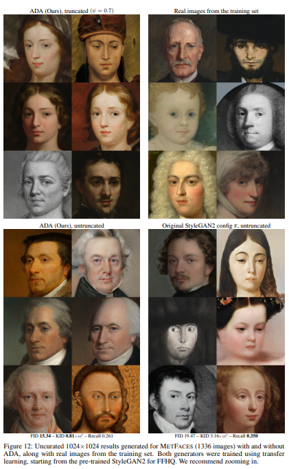
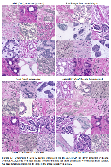
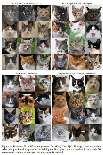
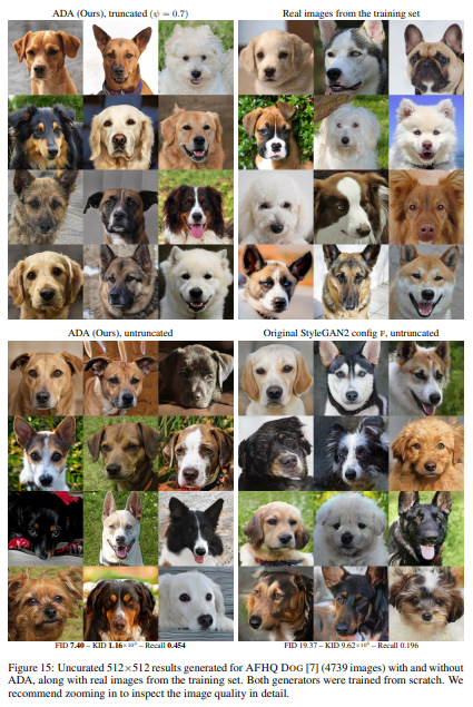
In Figures 12, 13, 14, 15, and 16, we show generated images for METFACES, BRECAHAD, and AFHQ CAT, DOG, WILD, respectively, along
with real images from the respective training sets (Section 4.3 and Figure 11a). The images were selected at random; we did not perform any cherrypicking besides choosing one global random seed. We can see that ADA yields excellent results in all cases, and with slight truncation [29, 20], virtually all of the images look convincing. Without ADA, the convergence is hampered by discriminator overfitting, leading to inferior image quality for the original StyleGAN2, especially in METFACES, AFHQ DOG, and BRECAHAD.
그림 12, 13, 14, 15 및 16에서는 METFACES, BRECAHAD 및 AFHQ CAT, DOG, WILD에 대해 각각 생성 된 이미지와 각 훈련 세트의 실제 이미지를 보여줍니다 (섹션 4.3 및 그림 11a). 이미지는 무작위로 선택되었습니다. 우리는 하나의 글로벌 랜덤 시드를 선택하는 것 외에 어떤 체리 피킹도 수행하지 않았습니다. 우리는 ADA가 모든 경우에서 우수한 결과를 산출하고 약간의 잘림 [29, 20]을 통해 사실상 모든 이미지가 설득력있게 보입니다. ADA가 없으면 판별 자 과적 합으로 수렴이 방해를 받아 원래 StyleGAN2, 특히 METFACES, AFHQ DOG 및 BRECAHAD에서 이미지 품질이 저하됩니다.
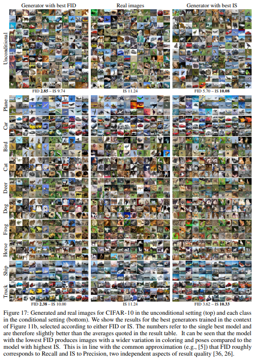
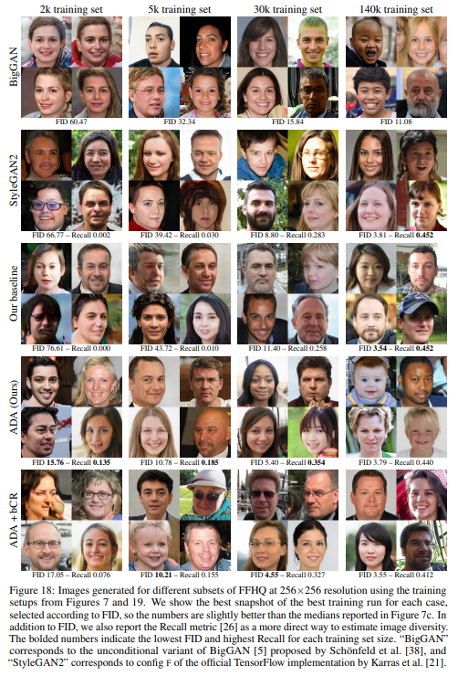
Figure 17 shows examples of the generated CIFAR-10 images in both unconditional and classconditional setting (See Appendix D.1 for details on the conditional setup). Figure 18 shows qualitative results for different methods using subsets of FFHQ at 256×256 resolution. Methods that do not employ augmentation (BigGAN, StyleGAN2, and our baseline) degrade noticeably as the size of the training set decreases, generally yielding poor image quality and diversity with fewer than 30k training images. With ADA, the degradation is much more graceful, and the results remain reasonable even with a 5k training set.
그림 17은 무조건 및 클래스 조건 설정 모두에서 생성 된 CIFAR-10 이미지의 예를 보여줍니다 (조건부 설정에 대한 자세한 내용은 부록 D.1 참조).
그림 18은 256x256 해상도에서 FFHQ의 하위 집합을 사용하는 다양한 방법에 대한 정 성적 결과를 보여줍니다.
증강을 사용하지 않는 방법 (BigGAN, StyleGAN2 및 기준)은 훈련 세트의 크기가 감소함에 따라 눈에 띄게 저하되며 일반적으로 3 만 개 미만의 훈련 이미지로 이미지 품질과 다양성이 저하됩니다. ADA를 사용하면 성능 저하가 훨씬 더 우아하고 결과는 5k 훈련 세트로도 합리적입니다.
Figure 19 compares our results with unconditional BigGAN [5, 38] and StyleGAN2 config F [21].
BigGAN was very unstable in our experiments: while some of the results were quite good, approximately 50% of the training runs failed to converge. StyleGAN2, on the other hand, behaved predictably, with different training runs resulting in nearly identical FID. We note that FID has a general tendency to increase as the training set gets smaller— not only because of the lower image quality, but also due to inherent bias in FID itself [3]. In our experiments, we minimize the impact of this bias by always computing FID between 50k generated images and all available real images, regardless of which subset was used for training. To estimate the magnitude of bias in FID, we simulate a hypothetical generator that replicates the training set as-is, and compute the average FID over 100 random trials with different subsets of training data; the standard deviation was ≤2% in all cases. We can see that the bias remains negligible with ≥20k training images but starts to dominate with ≤2k. Interestingly, ADA reaches the same FID as the best-case generator with FFHQ-1k, indicating that FID is no longer able to differentiate between the two in this case.
그림 19는 무조건 BigGAN [5, 38] 및 StyleGAN2 config F [21]의 결과를 비교합니다. BigGAN은 실험에서 매우 불안정했습니다. 일부 결과는 꽤 좋았지 만 훈련 실행의 약 50 %가 수렴하지 못했습니다. 반면 StyleGAN2는 서로 다른 훈련 실행으로 거의 동일한 FID를 생성하여 예측 가능하게 작동했습니다. FID는 학습 세트가 작아 질수록 증가하는 일반적인 경향이 있습니다. 이미지 품질이 낮을뿐만 아니라 FID 자체의 고유 한 편향 때문이기도합니다 [3]. 실험에서는 훈련에 사용 된 하위 집합에 관계없이 생성 된 50k 이미지와 사용 가능한 모든 실제 이미지 사이의 FID를 항상 계산하여이 편향의 영향을 최소화합니다. FID의 편향의 크기를 추정하기 위해 훈련 세트를있는 그대로 복제하는 가상 생성기를 시뮬레이션하고 훈련 데이터의 다른 하위 집합을 사용하여 100 번의 무작위 시도에 대한 평균 FID를 계산합니다. 표준 편차는 모든 경우에 ≤2 %였습니다. 20,000 개 이상의 트레이닝 이미지에서는 편향이 무시할 수 있지만 ≤2k로 우세하기 시작한다는 것을 알 수 있습니다. 흥미롭게도 ADA는 FFHQ-1k를 사용하는 최상의 경우 생성기와 동일한 FID에 도달하여이 경우 FID가 더 이상 둘을 구분할 수 없음을 나타냅니다.
Figure 20 shows additional examples of bCR leaking to generated images and compares bCR with dataset augmentation. In particular, rotations in range [−45◦ , +45◦ ] (denoted ±45◦ ) serve as a very clear example that attempting to make the discriminator blind to certain transformations opens up the possibility for the generator to produce similarly transformed images with no penalty. In applications where such leaks are acceptable, one can employ either bCR or dataset augmentation — we find that it is difficult to predict which method is better. For example, with translation augmentations bCR was significantly better than dataset augmentation, whereas x-flip was much more effective when implemented as a dataset augmentation.
그림 20은 생성 된 이미지로 유출되는 bCR의 추가 예를 보여주고 bCR을 데이터 세트 증가와 비교합니다. 특히 범위 [−45◦, + 45◦] (± 45◦로 표시)의 회전은 판별기를 특정 변환에 대해 차단하려고 시도하면 생성기가 다음과 같이 유사하게 변환 된 이미지를 생성 할 수있는 가능성을 열어주는 매우 명확한 예입니다. 벌금이 없습니다. 이러한 누출이 허용되는 애플리케이션에서는 bCR 또는 데이터 세트 증가를 사용할 수 있습니다. 어떤 방법이 더 나은지 예측하기가 어렵습니다. 예를 들어, 번역 증강을 사용하면 bCR이 데이터 세트 증강보다 훨씬 더 나은 반면, x-flip은 데이터 세트 증강으로 구현 될 때 훨씬 더 효과적이었습니다.
Finally, Figure 21 shows an extended version of Figure 4, illustrating the effect of different augmentation categories with increasing augmentation probability p. Blit + Geom + Color yielded the best results with a 2k training set and remained competitive with larger training sets as well.
마지막으로, 그림 21은 그림 4의 확장 버전을 보여 주며, 증가 확률 p가 증가함에 따라 다양한 증가 범주의 효과를 보여줍니다. Blit + Geom + Color는 2k 훈련 세트에서 최상의 결과를 얻었으며 더 큰 훈련 세트에서도 경쟁력을 유지했습니다.
B Our augmentation pipeline
We designed our augmentation pipeline based on three goals. First, the entire pipeline must be strictly non-leaking (Appendix C). Second, we aim for a maximally diverse set of augmentations, inspired by the success of RandAugment [9]. Third, we strive for the highest possible image quality to reduce unintended artifacts such as aliasing. In total, our pipeline consists of 18 transformations: geometric (7), color (5), filtering (4), and corruption (2). We implement it entirely on the GPU in a differentiable fashion, with full support for batching. All parameters are sampled independently for each image.
우리는 세 가지 목표를 기반으로 증강 파이프 라인을 설계했습니다. 첫째, 전체 파이프 라인은 엄격하게 누출되지 않아야합니다 (부록 C). 둘째, 우리는 RandAugment [9]의 성공에 영감을 받아 최대한 다양한 증강 세트를 목표로합니다. 셋째, 앨리어싱과 같은 의도하지 않은 아티팩트를 줄이기 위해 가능한 최고의 이미지 품질을 위해 노력합니다. 전체적으로 파이프 라인은 기하학적 (7), 색상 (5), 필터링 (4) 및 손상 (2)의 18 가지 변환으로 구성됩니다. 우리는 일괄 처리를 완벽하게 지원하여 차별화 가능한 방식으로 GPU에서 전적으로 구현합니다. 모든 매개 변수는 각 이미지에 대해 독립적으로 샘플링됩니다.
B.1 Geometric and color transformations 기하학적 및 색상 변환
Figure 22 shows pseudocode for our geometric and color transformations, along with example images. In general, geometric transformations tend to lose high-frequency details of the input image due to uneven resampling, which may reduce the capability of the discriminator to detect pixel-level errors in the generated images. We alleviate this by introducing a dedicated sub-category, pixel blitting, that only copies existing pixels as-is, without blending between neighboring pixels. Furthermore, we avoid gradual image degradation from multiple consecutive transformations by collapsing all geometric transformations into a single combined operation.
그림 22는 예제 이미지와 함께 기하학적 및 색상 변환에 대한 의사 코드를 보여줍니다. 일반적으로 기하학적 변환은 고르지 않은 리샘플링으로 인해 입력 이미지의 고주파 세부 정보를 잃는 경향이 있으며, 이는 생성 된 이미지에서 픽셀 수준 오류를 감지하는 판별 기의 기능을 감소시킬 수 있습니다. 인접한 픽셀을 혼합하지 않고 기존 픽셀 만 그대로 복사하는 전용 하위 범주 인 픽셀 블리 팅을 도입하여이를 완화합니다. 또한 모든 기하학적 변환을 단일 결합 작업으로 축소하여 여러 연속 변환으로 인한 점진적인 이미지 저하를 방지합니다.
The parameters for pixel blitting are selected on lines 5–15, consisting of x-flips (line 7), 90◦ rotations (line 10), and integer translations (line 13). The transformations are accumulated into a homogeneous 3 × 3 matrix G, defined so that input pixel (xi , yi) is placed at [xo, yo, 1]T = G · [xi , yi , 1]T in the output. The origin is located at the center of the image and neighboring pixels are spaced at unit intervals. We apply each transformation with probability p by sampling its parameters from uniform distribution, either discrete U{·} or continuous U(·), and updating G using elementary transforms: (2)
픽셀 블리 팅에 대한 매개 변수는 x-flip (7 행), 90 ° 회전 (10 행) 및 정수 변환 (13 행)으로 구성된 5-15 행에서 선택됩니다. 변환은 균질 한 3 × 3 행렬 G로 누적되며, 입력 픽셀 (xi, yi)이 출력에서 [xo, yo, 1] T = G · [xi, yi, 1] T에 배치되도록 정의됩니다. 원점은 이미지의 중앙에 있으며 인접 픽셀은 단위 간격으로 배치됩니다. 이산 U {·} 또는 연속 U (·)의 균일 분포에서 매개 변수를 샘플링하고 기본 변환을 사용하여 G를 업데이트하여 확률 p로 각 변환을 적용합니다. (2)
SCALE2D(sx, sy) = " sx 0 0 0 sy 0 0 0 1# , ROTATE2D(θ) = " cos θ − sin θ 0 sin θ cos θ 0 0 0 1# , TRANSLATE2D(tx, ty) = " 1 0 tx 0 1 ty 0 0 1 # (2)
General geometric transformations are handled in a similar way on lines 16–32, consisting of isotropic scaling (line 17), arbitrary rotation (lines 21 and 27), anisotropic scaling (line 24), and fractional translation (line 30). Since both of the scaling transformations are multiplicative in nature, we sample their parameter, s, from a log-normal distribution so that ln s ∼ N 0,(0.2 · ln 2)2 . In practice, this can be done by first sampling t ∼ N (0, 1) and then calculating s = exp2 (0.2t). We allow anisotropic scaling to operate in other directions besides the coordinate axes by breaking the rotation into two independent parts, one applied before the scaling (line 21) and one after it (line 27). We apply the rotations slightly less frequently than other transformations, so that the probability of applying at least one rotation is equal to p. Note that we also have two translations in our pipeline (lines 13 and 30), one applied at the beginning and one at the end. To increase the diversity of our augmentations, we use U(·) for the former and N (·) for the latter.
일반적인 기하학적 변환은 등방성 스케일링 (라인 17), 임의 회전 (라인 21 및 27), 비 등방성 스케일링 (라인 24) 및 부분 변환 (라인 30)으로 구성된 라인 16-32에서 유사한 방식으로 처리됩니다. 두 스케일링 변환은 본질적으로 곱하기 때문에 ln s ∼ N 0, (0.2 · ln 2) 2가되도록 로그 정규 분포에서 매개 변수 s를 샘플링합니다. 실제로 이것은 먼저 t ∼ N (0, 1)을 샘플링 한 다음 s = exp2 (0.2t)를 계산하여 수행 할 수 있습니다. 회전을 두 개의 독립적 인 부분으로 분할하여 비 등방성 스케일링이 좌표축 이외의 다른 방향으로 작동 할 수 있도록합니다. 하나는 스케일링 이전에 적용되고 (라인 21) 다른 하나는 이후에 적용됩니다 (라인 27). 회전을 다른 변환보다 약간 덜 자주 적용하므로 적어도 하나의 회전을 적용 할 확률은 p와 같습니다. 또한 파이프 라인에 두 개의 번역 (13 및 30 행)이 있습니다. 하나는 처음에 적용되고 다른 하나는 끝에 적용됩니다. 증강의 다양성을 높이기 위해 전자에 U (·)를 사용하고 후자에 N (·)을 사용합니다.
Once the parameters are settled, the combined geometric transformation is executed on lines 33–47. We avoid undesirable effects at image borders by first padding the image with reflection. The amount of padding is calculated dynamically based on G so that none of the output pixels are affected by regions outside the image (line 35). We then upsample the image to a higher resolution (line 40) and transform it using bilinear interpolation (line 45). Operating at a higher resolution is necessary to reduce aliasing when the image is minified, e.g., as a result of isotropic scaling— interpolating at the original resolution would fail to correctly filter out frequencies above Nyquist in this case, no matter which interpolation filter was used. The choice of the upsampling filter requires some care, however, because we must ensure that an identity transform does not modify the image in any way (e.g., when p = 0). In other words, we need to use a lowpass filter H(z) with cutoff fc = π 2 that satisfies DOWNSAMPLE2D UPSAMPLE2D Y, H(z −1 ) , H(z) = Y . Luckily, existing literature on wavelets [10] offers a wide selection of such filters; we choose 12-tap symlets (SYM6) to strike a balance between resampling quality and computational cost.
매개 변수가 정해지면 결합 된 기하학적 변환이 33-47 행에서 실행됩니다. 먼저 이미지를 반사로 패딩하여 이미지 테두리에서 원하지 않는 효과를 방지합니다. 패딩의 양은 G를 기반으로 동적으로 계산되므로 출력 픽셀은 이미지 외부 영역의 영향을받지 않습니다 (라인 35). 그런 다음 이미지를 더 높은 해상도 (라인 40)로 업 샘플링하고 쌍 선형 보간 (라인 45)을 사용하여 변환합니다. 예를 들어 등방성 스케일링의 결과로 이미지가 축소 될 때 앨리어싱을 줄이려면 더 높은 해상도에서 작동해야합니다.이 경우 원래 해상도로 보간하면 어떤 보간 필터가 사용되었는지에 관계없이 Nyquist 이상의 주파수를 올바르게 필터링하지 못합니다. . 그러나 업 샘플링 필터를 선택할 때는 약간의주의가 필요합니다. 왜냐하면 신원 변환이 어떤 방식으로도 이미지를 수정하지 않도록해야하기 때문입니다 (예 : p = 0 일 때). 즉, DOWNSAMPLE2D UPSAMPLE2D Y, H (z −1), H (z) = Y를 충족하는 컷오프 fc = π 2 인 저역 통과 필터 H (z)를 사용해야합니다. 다행히도 웨이블릿에 대한 기존 문헌 [10]은 이러한 필터의 다양한 선택을 제공합니다. 리샘플링 품질과 계산 비용 간의 균형을 맞추기 위해 12 탭 symlet (SYM6)을 선택합니다.
Finally, color transformations are applied to the resulting image on lines 48–70. The overall operation is similar to geometric transformations: we collect the parameters of each individual transformation into a homogeneous 4 × 4 matrix C that we then apply to each pixel by computing [ro, go, bo, 1]T = C · [ri , gi , bi , 1]T . The transformations include adjusting brightness (line 50), contrast (line 53), and saturation (line 63), as well as flipping the luma axis while keeping the chroma unchanged (line 57) and rotating the hue axis by an arbitrary amount (line 60).
마지막으로 48 ~ 70 행의 결과 이미지에 색상 변환이 적용됩니다. 전체 작업은 기하학적 변환과 유사합니다. 각 개별 변환의 매개 변수를 동종 4 × 4 행렬 C로 수집 한 다음 [ro, go, bo, 1] T = C · [ri, gi, bi, 1] T. 변환에는 밝기 (라인 50), 대비 (라인 53) 및 채도 (라인 63) 조정, 채도를 변경하지 않고 (라인 57) 색조 축을 임의의 양만큼 회전 (라인 60).
B.2 Image-space filtering and corruptions 이미지 공간 필터링 및 손상
Figure 23 shows pseudocode for our image-space filtering and corruptions. The parameters for image space filtering are selected on lines 5–14. The idea is to divide the frequency content of the image into 4 non-overlapping bands and amplify/weaken each band in turn via a sequence of 4 transformations, so that each transformation is applied independently with probability p (lines 9–10). Frequency bands b2, b3, and b4 correspond to the three highest octaves, respectively, while the remaining low frequencies are attributed to b1 (line 6). We track the overall gain of each band using vector g (line 7) that we update after each transformation (line 14). We sample the amplification factor for a given band from log-normal distribution (line 12), similar to geometric scaling, and normalize the overall gain so that the total energy is retained on expectation. For the normalization, we assume that the frequency content obeys 1/f power spectrum typically seen in natural images (line 8). While this assumption is not strictly true in our case, especially when some of the previous frequency bands have already been amplified, it is sufficient to keep the output pixel values within reasonable bounds.
그림 23은 이미지 공간 필터링 및 손상에 대한 의사 코드를 보여줍니다. 이미지 공간 필터링을위한 매개 변수는 라인 5-14에서 선택됩니다. 아이디어는 이미지의 주파수 내용을 4 개의 겹치지 않는 밴드로 나누고 4 개의 변환 시퀀스를 통해 차례로 각 밴드를 증폭 / 약화시켜 각 변환이 확률 p (9-10 행)로 독립적으로 적용되도록하는 것입니다. 주파수 대역 b2, b3 및 b4는 각각 가장 높은 세 옥타브에 해당하고 나머지 저주파는 b1 (6 행)에 해당합니다. 각 변환 (14 행) 후 업데이트하는 벡터 g (7 행)를 사용하여 각 대역의 전체 이득을 추적합니다. 기하학적 스케일링과 유사한 로그 정규 분포 (라인 12)에서 주어진 대역에 대한 증폭 계수를 샘플링하고 총 에너지가 예상대로 유지되도록 전체 이득을 정규화합니다. 정규화를 위해 주파수 성분이 일반적으로 자연 이미지에서 볼 수있는 1 / f 전력 스펙트럼을 따른다고 가정합니다 (8 행). 이 가정은 우리의 경우, 특히 이전 주파수 대역 중 일부가 이미 증폭 된 경우에는 엄격히 사실이 아니지만 출력 픽셀 값을 합리적인 범위 내로 유지하는 것으로 충분합니다.
The filtering is executed on lines 15–23. We first construct a combined amplification filter H0 (z) (lines 17–19) and then perform separable convolution for the image using reflection padding (lines 21– 23). We use a zero-phase filter bank derived from 4-tap symlets (SYM2) [10]. Denoting the wavelet scaling filter by H(z), the corresponding bandpass filters are obtained as follows (line 19):
필터링은 15-23 행에서 실행됩니다. 먼저 결합 된 증폭 필터 H0 (z) (17 ~ 19 행)을 구성한 다음 반사 패딩 (21 ~ 23 행)을 사용하여 이미지에 대해 분리 가능한 회선을 수행합니다. 4 탭 symlet (SYM2)에서 파생 된 영 위상 필터 뱅크를 사용합니다 [10]. 웨이블릿 스케일링 필터를 H (z)로 표시하면 해당 대역 통과 필터가 다음과 같이 얻어집니다 (19 행).
Finally, we apply additive RGB noise on lines 24–29 and cutout on lines 30–35. We vary the strength of the noise by sampling its standard deviation from half-normal distribution, i.e., N (·) restricted to non-negative values (line 26). For cutout, we match the original implementation of DeVries and Taylor [11] by setting pixels to zero within a rectangular area of size w 2 , h 2 , with the center point selected from uniform distribution over the entire image.
마지막으로 24 ~ 29 행에 추가 RGB 노이즈를 적용하고 30 ~ 35 행에 컷 아웃을 적용합니다. 정규 분포의 절반, 즉 음이 아닌 값으로 제한된 N (·) (26 행)에서 표준 편차를 샘플링하여 노이즈의 강도를 변경합니다. 컷 아웃의 경우, 전체 이미지에 대한 균일 한 분포에서 선택된 중심점을 사용하여 크기 w 2, h 2의 직사각형 영역 내에서 픽셀을 0으로 설정하여 DeVries 및 Taylor [11]의 원래 구현과 일치시킵니다.
C Non-leaking augmentations 비누출 증가
The goal of GAN training is to find a generator function G whose output probability distribution x (under suitable stochastic input) matches a given target distribution y.
GAN 훈련의 목표는 출력 확률 분포 x (적절한 확률 적 입력에서)가 주어진 목표 분포 y와 일치하는 생성기 함수 G를 찾는 것입니다
When augmenting both the dataset and the generator output, the key safety principle is that if x and y do not match, then their augmented versions must not match either. If the augmentation pipeline violates this principle, the generator is free to learn some different output distribution than the dataset, as these look identical after the augmentations – we say that the augmentations leak. Conversely, if the principle holds, then the only option for the generator is to learn the correct distribution: no other choice results in a post-augmentation match.
데이터 세트와 생성기 출력을 모두 증가시킬 때 주요 안전 원칙은 x와 y가 일치하지 않으면 해당 증가 버전도 일치하지 않아야한다는 것입니다. 증강 파이프 라인이이 원칙을 위반하는 경우 생성기는 데이터 세트와 다른 출력 분포를 자유롭게 학습 할 수 있습니다. 이는 증강 후 동일 해 보이기 때문입니다. 우리는 증강이 누출된다고 말합니다. 반대로 원칙이 유지되는 경우 생성기의 유일한 옵션은 올바른 분포를 배우는 것입니다. 다른 선택은 증가 후 일치를 초래하지 않습니다.
In this section, we study the conditions on the augmentation pipeline under which this holds and demonstrate the safety and caveats of various common augmentations and their compositions.
이 섹션에서는 다양한 일반적인 증강 및 그 구성의 안전성과주의 사항을 유지하고 입증하는 증강 파이프 라인의 조건을 연구합니다.
표기법이 섹션 전체에서 소문자 굵은 글씨 (예 : x)를 사용하는 확률 분포 (및 일반화), 붓글씨 (T)로 작업하는 연산자, 대문자 (X)로 확률 분포에서 샘플링 된 변수를 표시합니다. ).
Notation Throughout this section, we denote probability distributions (and their generalizations) with lowercase bold-face letters (e.g., x), operators acting on them by calligraphic letters (T ), and variates sampled from probability distributions by upper-case letters (X).
표기법이 섹션에서는 소문자 굵은 글씨체 (예 : x)를 사용하는 확률 분포 (및 일반화), 붓글씨 (T)로 작동하는 연산자, 대문자 (X)로 확률 분포에서 샘플링 한 변수를 표시합니다. ).
C.1 Augmentation operator 증강 연산자
A very general model for augmentations is as follows. Assume a fixed but arbitrarily complicated nonlinear and stochastic augmentation pipeline. To any image X, it assigns a distribution of augmented images, such as demonstrated in Figure 2c. This idea is captured by an augmentation operator T that maps probability distributions to probability distributions (or, informally, datasets to augmented datasets). A distribution with the lone image X is the Dirac point mass δX, which is mapped to some distribution T δX of augmented images.3 In general, applying T to an arbitrary distribution x yields the linear superposition T x of such augmented distributions.
증강에 대한 매우 일반적인 모델은 다음과 같습니다. 고정되었지만 임의적으로 복잡한 비선형 및 확률 적 증대 파이프 라인을 가정합니다. 모든 이미지 X에 그림 2c와 같이 증강 이미지의 분포를 할당합니다. 이 아이디어는 확률 분포를 확률 분포 (또는 비공식적으로 데이터 세트를 증강 데이터 세트로)로 매핑하는 증강 연산자 T에 의해 포착됩니다. 고독한 이미지 X가있는 분포는 Dirac 포인트 질량 δX이며, 이는 증강 이미지의 일부 분포 T δX에 매핑됩니다 .3 일반적으로 임의 분포 x에 T를 적용하면 이러한 증강 분포의 선형 중첩 T x가 생성됩니다.
It is important to understand that T is different from a function f(X; φ) that actually applies the augmentation on any individual image X sampled from x (parametrized by some φ, e.g., angle in case of a rotation augmentation). It captures the aggregate effect of applying this function on all images in the distribution and subsumes the randomization of the function parameters. T is always linear and deterministic, regardless of non-linearity of the function f and stochasticity of its parameters φ. We will later discuss invertibility of T . Here it is also critical to note that its invertibility is not equivalent with the invertibility of the function f it is based on; for an example, refer to the discussion in Section 2.2.
T는 x에서 샘플링 된 개별 이미지 X에 실제로 증가를 적용하는 함수 f (X; φ)와 다르다는 것을 이해하는 것이 중요합니다 (예 : 회전 증가의 경우 각도에 의해 일부 φ로 매개 변수화 됨). 분포의 모든 이미지에이 함수를 적용한 집계 효과를 캡처하고 함수 매개 변수의 무작위 화를 포함합니다. T는 함수 f의 비선형 성과 매개 변수 φ의 확률성에 관계없이 항상 선형적이고 결정적입니다. 나중에 T의 가역성에 대해 논의 할 것입니다. 여기에서 그것의 가역성은 그것이 기반으로하는 함수 f의 가역성과 동일하지 않다는 점에 유의하는 것이 중요합니다. 예를 들어 섹션 2.2의 설명을 참조하십시오.
Specifically, T is a (Markov) transition operator. Intuitively, it is an (uncountably) infinitedimensional generalization of a Markov transition matrix (i.e. a stochastic matrix), with nonnegative entries that sum to 1 along columns. In this analogy, probability distributions upon which T operates are vectors, with nonnegative entries summing to 1. More generally, the distributions have a vector space structure and they can be arbitrarily linearly combined (in which case they may lose their validity as probability distributions and are viewed as arbitrary signed measures). Similarly, we can do algebra with the with the operators by linearly combining and composing them like matrices. Concepts such as null space and invertibility carry over to this setting, with suitable technical care. In the following, we will be somewhat informal with the measure theoretical and functional analytic details of the problem, and draw upon this analogy as appropriate.
특히 T는 (Markov) 전환 연산자입니다. 직관적으로, 이것은 열을 따라 합이 1이되는 음이 아닌 항목을 가진 마르코프 전이 행렬 (즉, 확률 행렬)의 무한 차원 일반화입니다. 이 비유에서 T가 작동하는 확률 분포는 음이 아닌 항목의 합계가 1 인 벡터입니다.보다 일반적으로 분포는 벡터 공간 구조를 가지며 임의로 선형 결합 될 수 있습니다 (이 경우 확률 분포 및 임의의 서명 된 측정 값으로 간주 됨). 마찬가지로 연산자를 행렬처럼 선형 결합하고 구성하여 연산자를 사용하여 대수를 수행 할 수 있습니다. 널 공간 및 가역성과 같은 개념은 적절한 기술 관리와 함께이 설정으로 이어집니다. 다음에서, 우리는 문제의 이론적 및 기능적 분석 세부 사항에 대해 다소 비공식적이며 적절하게이 비유를 그릴 것입니다.
C.2 Invertibility implies non-leaking augmentations 가역성은 비누출 증가를 의미합
Within this framework, our question can be stated as follows. Given a target distribution y and an augmentation operator T , we train for a generated distribution x such that the augmented distributions match, namely
이 틀 안에서 우리의 질문은 다음과 같이 말할 수 있습니다. 목표 분포 y와 증가 연산자 T가 주어지면, 우리는 생성 된 분포 x에 대해 증가 된 분포가 일치하도록 훈련합니다.
T x = T y. (7)
The desired outcome is that this equation is satisfied only by the correct target distribution, namely x = y. We say that T leaks if there exist distributions x 6= y that satisfy the above equation, and the goal is to find conditions that guarantee the absence of leaks.
There are obviously no such leaks in classical non-augmented training, where T is the identity I, whence T x = T y ⇒ Ix = Iy ⇒ x = y. For arbitrary augmentations, the desired outcome x = y does always satisfy Eq. 7; however, if also other choices of x satisfy it, then it cannot be guaranteed that the training lands on the desired solution. A trivial example is an augmentation that maps every image to black (in other words, T z = δ0 for any z). Then, T x = T y does not imply that x = y, as indeed any choice of x produces the same set of black images that satisfies Eq. 7. In this case, it is vanishingly unlikely that the training finds the solution x = y.
원하는 결과는이 방정식이 올바른 목표 분포, 즉 x = y에 의해서만 충족된다는 것입니다. 위의 방정식을 만족하는 분포 x 6 = y가 존재하면 T가 누출된다고 말하며, 목표는 누출이 없음을 보장하는 조건을 찾는 것입니다. 고전적인 비 증강 훈련에는 분명히 그러한 누출이 없습니다. 여기서 T는 정체성 I이고, 여기서 T x = T y ⇒ Ix = Iy ⇒ x = y입니다. 임의의 증가의 경우 원하는 결과 x = y는 항상 Eq를 충족합니다. 7; 그러나 x의 다른 선택도 만족한다면 훈련이 원하는 솔루션에 도달한다고 보장 할 수 없습니다. 간단한 예는 모든 이미지를 검은 색으로 매핑하는 증강입니다 (즉, 모든 z에 대해 T z = δ0). 그러면 T x = T y는 x = y를 의미하지 않습니다. 실제로 x를 선택하면 Eq를 충족하는 동일한 검정 이미지 세트가 생성됩니다. 7.이 경우 훈련이 해 x = y를 찾을 가능성은 거의 없습니다.
More generally, assume that T has a non-trivial null space, namely there exists a signed measure n 6= 0 such that T n = 0, that is, n is in the null space of T . Equivalently, T is not invertible, because n cannot be recovered from T n. Then, x = y + αn for any α ∈ R satisfies Eq. 7. Therefore noninvertibility of T implies that measures in its null space may freely leak into the learned distribution (as long as the sum remains a valid probability distribution that assigns non-negative mass to all sets). Conversely, assume that some x 6= y satisfies Eq. 7. Then T (x − y) = T y − T y = 0, so x − y is in null space of T and therefore T is not invertible.
보다 일반적으로, T가 사소하지 않은 널 공간을 가지고 있다고 가정합니다. 즉, T n = 0, 즉 n이 T의 널 공간에있는 부호있는 측정 값 n 6 = 0이 존재합니다. 마찬가지로, n은 T n에서 복구 할 수 없기 때문에 T는 가역적이지 않습니다. 그러면 α ∈ R에 대한 x = y + αn은 Eq를 충족합니다. 7. 따라서 T의 비가역성은 null 공간의 측정 값이 학습 된 분포로 자유롭게 누출 될 수 있음을 의미합니다 (합이 모든 집합에 음이 아닌 질량을 할당하는 유효한 확률 분포로 유지되는 한). 반대로 일부 x 6 = y가 Eq를 충족한다고 가정합니다. 7. 그러면 T (x − y) = T y − T y = 0이므로 x − y는 T의 영 공간에 있으므로 T는 반전 할 수 없습니다.
Therefore, leaking augmentations imply non-invertibility of the augmentation operator, which conversely implies the central principle: if the augmentation operator T is invertible, it does not leak. Such a non-leaking operator further satisfies the requirements of Lemma 5.1. of Bora et al. [4], where the invertibility is shown to imply that a GAN learns the correct distribution.
따라서 누출 증가는 증가 연산자의 비가역성을 의미하며, 이는 반대로 중심 원칙을 의미합니다. 증가 연산자 T가 가역적이면 누출되지 않습니다. 이러한 비누출 연산자는 Lemma 5.1의 요구 사항을 추가로 충족합니다. of Bora et al. [4], 가역성은 GAN이 올바른 분포를 학습 함을 의미하는 것으로 표시됩니다.
The invertibility has an intuitive interpretation: the training process can implicitly “undo” the augmentations, as long as probability mass is merely shifted around and not squashed flat.
가역성에는 직관적 인 해석이 있습니다. 확률 질량이 평평하게 찌그러지지 않고 단순히 이동하는 한, 훈련 과정은 암시 적으로 증강을 "실행 취소"할 수 있습니다.
C.3 Compositions and mixtures
We only access the operator T indirectly: it is implemented as a procedure, rather than a matrix-like entity whose null space we could study directly (even if we know that such a thing exists in principle). Showing invertibility for an arbitrary procedure is likely to be impossible. Rather, we adopt a constructive approach, and build our augmentation pipeline from combinations of simple known-safe augmentations, in a way that can be shown to not leak. This calls for two components: a set of combination rules that preserve the non-leaking guarantee, and a set of elementary augmentations that have this property. In this subsection we address the former.
우리는 연산자 T에 간접적으로 만 접근합니다. 그것은 우리가 직접 연구 할 수있는 행렬과 같은 개체가 아니라 절차로 구현됩니다 (원칙적으로 그러한 것이 존재한다는 것을 알고 있더라도). 임의의 절차에 대해 가역성을 보여주는 것은 불가능할 수 있습니다. 오히려 우리는 건설적인 접근 방식을 채택하고, 누출되지 않는 것으로 보일 수있는 방식으로 알려진 안전하고 단순한 증강의 조합에서 증강 파이프 라인을 구축합니다. 이를 위해서는 두 가지 구성 요소가 필요합니다. 비누 출 보장을 유지하는 조합 규칙 집합과이 속성이있는 기본 확장 집합입니다. 이 하위 섹션에서는 전자를 다룹니다.
By elementary linear algebra: assume T and U are invertible. Then the composition T U is invertible, as is any finite chain of such compositions. Hence, sequential composition of non-leaking augmentations is non-leaking. We build our pipeline on this observation.
기본 선형 대수 : T와 U가 가역적이라고 가정합니다. 그런 다음 구성 T U는 그러한 구성의 유한 체인과 마찬가지로 가역적입니다. 따라서, 비누 출 증가의 순차적 구성은 비누 수입니다. 우리는이 관찰을 바탕으로 파이프 라인을 구축합니다.
The other obvious combination of augmentations is obtained by probabilistic mixtures: given invertible augmentations T and U, perform T with probability α and U with probability 1 − α. The operator corresponding to this augmentation is the “pointwise” convex blend αT + (1 − α)U. More generally, one can mix e.g. a continuous family of augmentations Tφ with weights given by a non-negative unit-sum function α(φ), as R α(φ)Tφ dφ. Unfortunately, stochastically choosing among a set of augmentations is not guaranteed to preserve the non-leaking property, and must be analyzed case by case (which is the content of the next subsection). To see this, consider an extremely simple discrete probability space with only two elements. The augmentation operator T = 0 1 1 0 flips the elements. Mixed with probability α = 1 2 with the identity augmentation I (which keeps the distribution unchanged), we obtain the augmentation 1 2 T + 1 2 I = 1 2 1 1 1 1 which is a singular matrix and therefore not invertible. Intuitively, this operator smears any probability distribution into a degenerate equidistribution, from which the original can no longer be recovered. Similar considerations carry over to arbitrarily complicated linear operators.
다른 명백한 증가 조합은 확률 적 혼합에 의해 얻어집니다. 가역적 증가 T와 U가 주어지면 확률 α로 T를 수행하고 확률 1 − α로 U를 수행합니다. 이 증가에 해당하는 연산자는 "점별"볼록 혼합 αT + (1 − α) U입니다. 더 일반적으로, 예를 들어 혼합 할 수 있습니다. R α (φ) Tφ dφ와 같이 음이 아닌 단위 합 함수 α (φ)에 의해 주어진 가중치를 갖는 연속 증가 군 Tφ. 안타깝게도 일련의 확장 중에서 확률 적으로 선택하는 것은 비누 출 속성을 보존한다고 보장 할 수 없으며 사례별로 분석해야합니다 (다음 하위 섹션의 내용). 이를 확인하기 위해 두 개의 요소 만있는 매우 단순한 이산 확률 공간을 고려하십시오. 증가 연산자 T = 0 1 1 0은 요소를 뒤집습니다. 확률 α = 1 2와 동일성 증가 I (분포를 변경하지 않은 상태로 유지)와 혼합하면 단일 행렬이므로 가역적이지 않은 증가 1 2 T + 1 2 I = 1 2 1 1 1 1을 얻습니다. 직관적으로이 연산자는 확률 분포를 퇴화 등분 포로 번져서 원본을 더 이상 복구 할 수 없습니다. 유사한 고려 사항이 임의로 복잡한 선형 연산자에도 적용됩니다.
C.4 Non-leaking elementary augmentations 비누출 기초 증강
In the following, we construct several examples of relatively large classes of elementary augmentations that do not leak and can therefore be used to form a chain of augmentations. Importantly, most of these classes are not inherently safe, as they are stochastic mixtures of even simpler augmentations, as discussed above. However, in many cases we can show that the degenerate situation only arises with specific choices of mixture distribution, which we can then avoid.
다음에서, 우리는 누출되지 않으므로 증강 체인을 형성하는 데 사용할 수있는 비교적 큰 클래스의 기본 증강의 몇 가지 예를 구성합니다. 중요한 것은, 이러한 클래스의 대부분은 위에서 논의한 것처럼 더 단순한 증가의 확률 적 혼합물이기 때문에 본질적으로 안전하지 않습니다. 그러나 많은 경우에 우리는 퇴화 상황이 혼합물 분포의 특정 선택에서만 발생한다는 것을 보여줄 수 있습니다.
Specifically, for every type of augmentation, we identify a configuration where applying it with probability strictly less than 1 results in an invertible transformation. From the standpoint of this analysis, we interpret this stochastic skipping as modifying the augmentation operator itself, in a way that boosts the probability of leaving the input unchanged and reduces the probability of other outcomes.
특히 모든 유형의 증강에 대해 엄격하게 1 미만의 확률로 적용하면 역변환이 발생하는 구성을 식별합니다. 이 분석의 관점에서, 우리는이 확률 적 건너 뛰기를 입력을 변경하지 않고 그대로 둘 가능성을 높이고 다른 결과의 가능성을 줄이는 방식으로 증가 연산자 자체를 수정하는 것으로 해석합니다.
C.4.1 Deterministic mappings 결정적 매핑
The simplest form of augmentation is a deterministic mapping, where the operator Tf assigns to every image X a unique image f(X). In the most general setting f is any measurable function and Tfx is the corresponding pushforward measure. When f is a diffeomorphism, Tf acts by the usual change of variables formula with a density correction by a Jacobian determinant. These mappings are invertible as long as f itself is invertible. Conversely, if f is not invertible, then neither is Tf .
가장 간단한 형태의 증강은 결정 론적 매핑으로, 연산자 Tf는 모든 이미지 X에 고유 한 이미지 f (X)를 할당합니다. 가장 일반적인 설정에서 f는 측정 가능한 함수이고 Tfx는 해당 푸시 포워드 측정입니다. f가 diffeomorphism이면 Tf는 Jacobian 행렬식에 의한 밀도 보정을 사용하여 변수 공식의 일반적인 변경에 따라 작동합니다. 이러한 매핑은 f 자체가 가역적이면 가역적입니다. 반대로 f가 가역적이지 않으면 Tf도 마찬가지입니다.
Here it may be instructive to highlight the difference between f and Tf . The former transforms the underlying space on which the probability distributions live – for example, if we are dealing with images of just two pixels (with continuous and unconstrained values), f is a nonlinear “warp” of the two-dimensional plane. In contrast, Tf operates on distributions defined on this space – think of a continuous 2-dimensional function (density) on the aforementioned plane. The action of Tf is to move the density around according to f, while compensating for thinning and concentration of the mass due to stretching. As long as f maps every distinct point to a distinct point, this warp can be reversed.
여기서 f와 Tf의 차이점을 강조하는 것이 도움이 될 수 있습니다. 전자는 확률 분포가 존재하는 기본 공간을 변환합니다. 예를 들어 단 2 픽셀의 이미지 (연속 및 제한되지 않은 값 포함)를 처리하는 경우 f는 2 차원 평면의 비선형 "왜곡"입니다. 반대로 Tf는이 공간에 정의 된 분포에서 작동합니다. 앞서 언급 한 평면에서 연속적인 2 차원 함수 (밀도)를 생각해보십시오. Tf의 작용은 f에 따라 밀도를 이동하는 동시에 스트레칭으로 인한 질량의 얇아 짐과 집중을 보상하는 것입니다. f가 모든 고유 지점을 고유 지점에 매핑하는 한이 뒤틀림은 반전 될 수 있습니다.
An important special case is that where f is a linear transformation of the space. Then the invertibility of Tf becomes a simpler question of the invertibility of a finite-dimensional matrix that represents f.
중요한 특별한 경우는 f가 공간의 선형 변환 인 경우입니다. 그러면 Tf의 가역성은 f를 나타내는 유한 차원 행렬의 가역성에 대한 더 간단한 질문이됩니다.
Note that when an invertible deterministic transformation is skipped probabilistically, the determinism is lost, and very specific choices of transformation could result in non-invertibility (see e.g. the example of flipping above). We only use deterministic mappings as building blocks of other augmentations, and never apply them in isolation with stochastic skipping.
가역적 결정 론적 변환을 확률 적으로 건너 뛰면 결정론이 손실되고 매우 특정한 변환 선택으로 인해 비가역성이 발생할 수 있습니다 (예 : 위의 뒤집기 예제 참조). 우리는 결정 론적 매핑을 다른 확장의 구성 요소로만 사용하고 확률 적 건너 뛰기와 격리하여 적용하지 않습니다.
C.4.2 Transformation group augmentations 변환 그룹 증가
Many commonly used augmentations are built from transformations that act as a group under sequential composition. Examples of this are flips, translations, rotations, scalings, shears, and many color and intensity transformations. We show that a stochastic mixture of transformations within a finitely generated abelian group is non-leaking as long as the mixture weights are chosen from a non-degenerate distribution.
일반적으로 사용되는 많은 증강은 순차적 구성에서 그룹 역할을하는 변환에서 작성됩니다. 이것의 예로는 뒤집기, 평행 이동, 회전, 크기 조절, 가위 및 다양한 색상 및 강도 변형이 있습니다. 유한하게 생성 된 아벨 그룹 내에서 확률 론적 변환 혼합은 혼합 가중치가 비 퇴화 분포에서 선택되는 한 누출되지 않음을 보여줍니다.
As an example, the four deterministic augmentations {R0, R90, R180, R270} that rotate the images to every one of the 90-degree increment orientations constitute a group. This is seen by checking that the set satisfies the axiomatic definition of a group. Specifically, the set is closed, as composing two of elements always results in an element of the same set, e.g. R270R180 = R90. It is also obviously associative, and has an identity element R0 = I. Finally, every element has an inverse, e.g. R −1 90 = R270. We can now simply speak of powers of the single generator element, whereby the four group elements are written as {R0 90, R1 90, R2 90, R3 90} and further (as well as negative) powers “wrap over” to the same elements. This group is isomorphic to Z4, the additive group of integers modulo 4.
예를 들어, 이미지를 90도 증분 방향으로 회전시키는 4 개의 결정 론적 증강 {R0, R90, R180, R270}이 그룹을 구성합니다. 이는 세트가 그룹의 공리적 정의를 충족하는지 확인하여 알 수 있습니다. 특히, 두 개의 요소를 구성하면 항상 동일한 세트의 요소가 생성되므로 세트가 닫힙니다. R270R180 = R90입니다. 또한 분명히 연관성이 있으며 동일 요소 R0 = I를 갖습니다. 마지막으로 모든 요소에는 역이 있습니다. R -1 90 = R270. 이제 단일 발전기 요소의 거듭 제곱에 대해 간단히 말할 수 있습니다. 그러면 4 개의 그룹 요소가 {R0 90, R1 90, R2 90, R3 90}로 작성되고 더 많은 (음수뿐 아니라) 거듭 제곱이 동일한 것에 "랩 오버"됩니다. 집단. 이 그룹은 모듈로 4 인 정수의 추가 그룹 인 Z4와 동형입니다.
A group of rotations is compact due to the wrap-over effect. An example of a non-compact group is that of translations (with non-periodic boundary conditions): compositions of translations are still translations, but one cannot wrap over. Furthermore, more than one generator element can be present (e.g. y-translation in addition to x-translation), but we require that these commute, i.e. the order of applying the transformations must not matter (in which case the group is called abelian).
랩 오버 효과로 인해 회전 그룹이 콤팩트합니다. 압축되지 않은 그룹의 예로는 번역 (비 주기적 경계 조건 포함)이 있습니다. 번역의 구성은 여전히 번역이지만 하나는 마무리 할 수 없습니다. 또한 생성기 요소가 두 개 이상있을 수 있지만 (예 : x- 변환에 추가하여 y- 변환), 이러한 통근이 필요합니다. 즉, 변환을 적용하는 순서는 중요하지 않아야합니다 (이 경우 그룹을 아벨이라고 함). .
Similar considerations extend to continuous Lie groups, e.g. that of rotations by any angle; here the generating element is replaced by an infinitesimal generator from the corresponding Lie algebra, and the discrete powers by the continuous exponential mapping. For example, continuous rotation transformations are isomorphic to the group SO(2), or U(1).
유사한 고려 사항이 연속 거짓말 그룹으로 확장됩니다. 모든 각도에 의한 회전; 여기서 생성 요소는 해당 거짓말 대수에서 무한소 생성기로 대체되고 이산 거듭 제곱은 연속 지수 매핑으로 대체됩니다. 예를 들어 연속 회전 변환은 그룹 SO (2) 또는 U (1)과 동형입니다.
In the following subsections show that for finitely generated abelian groups whose identity element matches the identity augmentation, stochastic mixtures of augmentations within the group are invertible, as long as the appropriate Fourier transform of the probability distribution over the elements has no zeros.
다음 하위 섹션에서, 동일성 요소가 동일성 증가와 일치하는 유한하게 생성 된 아벨 그룹의 경우, 요소에 대한 확률 분포의 적절한 푸리에 변환에 0이없는 한 그룹 내에서 증가의 확률 적 혼합이 반전 될 수 있음을 보여줍니다.
Discrete compact one-parameter groups We demonstrate the key points in detail with the simple but relevant case of a discrete compact one-parameter group and generalize later. Let G be a deterministic augmentation that generates the finite cyclic group {Gi} N−1 i=0 of order N (e.g. the four 90-degree rotations above), such that the element G 0 is the identity mapping that leaves its input unchanged.
이산 형 콤팩트 1- 파라미터 그룹 이산 형 콤팩트 1- 파라미터 그룹의 단순하지만 관련성있는 사례를 통해 핵심 사항을 자세히 설명하고 나중에 일반화합니다. G를 N 차 (예 : 위의 4 개의 90도 회전)의 유한 순환 그룹 {Gi} N−1 i = 0을 생성하는 결정 론적 증가라고 가정합니다. 따라서 요소 G 0은 입력을 변경하지 않은 ID 매핑입니다. .
Consider a stochastic augmentation T that randomly applies an element of the group, with the probability of choosing each element given by the probability vector p ∈ R N (where p is nonnegative and sums to 1): T = N X−1 i=0 piG i (8)
To show the conditions for invertibility of T , we build an operator U that explicitly inverts T , namely UT = I = G 0 . Whenever this is possible, T is invertible and non-leaking. We build U from the same group elements with a different weighting5 vector q ∈ R N : U = N X−1 j=0 qjG j (9)
We now seek a vector q for which UT = I, that is, for which U is the desired inverse. Now,
확률 벡터 p ∈ RN (p는 음이 아니고 합이 1)에 의해 주어진 각 요소를 선택할 확률과 함께 그룹의 요소를 무작위로 적용하는 확률 적 증가 T를 고려하십시오. T = NX−1 i = 0 piG i (8) T의 가역성 조건을 표시하기 위해 명시 적으로 T를 반전하는 연산자 U, 즉 UT = I = G 0을 만듭니다. 이것이 가능할 때마다 T는 가역적이며 누출되지 않습니다. 가중치가 다른 동일한 그룹 요소에서 U를 만듭니다 .5 벡터 q ∈ R N : U = N X−1 j = 0 qjG j (9) 이제 우리는 UT = I, 즉 U가 원하는 역인 벡터 q를 찾습니다. 지금,
UT = N X−1 i=0 piG i ! N X−1 j=0 qjG j (10)
= N X−1 i,j=0 piqjG i+j (11)
The powers of the group operation, as well as the indices of the weight vectors, are taken as modulo N due to the cyclic wrap-over of the group element. Collecting the terms that correspond to each G k in this range and changing the indexing accordingly, we arrive at:
그룹 연산의 거듭 제곱과 가중치 벡터의 인덱스는 그룹 요소의 순환 랩 오버로 인해 모듈로 N으로 간주됩니다. 이 범위의 각 G k에 해당하는 항을 수집하고 그에 따라 색인을 변경하면 다음과 같은 결과에 도달합니다.
(12)
(13)
where we observe that the multiplier in front of each G k is given by the cyclic convolution of the elements of the vectors p and q. This can be written as a pointwise product in terms of the Discrete Fourier Transform F, denoting the DFT’s of p and q by a hat:
여기서 우리는 각 G k 앞의 승수가 벡터 p와 q 요소의 순환 컨볼 루션에 의해 주어집니다. 이것은 모자로 p와 q의 DFT를 나타내는 Discrete Fourier Transform F의 관점에서 점적 곱으로 작성할 수 있습니다.
(14)
To recover the sought after inverse, assuming every element of pˆ is nonzero, we set qˆi = 1 pˆi for all i:
pˆ의 모든 요소가 0이 아니라고 가정하고 구한 역을 복구하기 위해 모든 i에 대해 qˆi = 1 pˆi를 설정합니다.
(15)(16)(17)(18)
Here, we take advantage of the fact that the inverse DFT of a constant vector of ones is the vector [1, 0, ..., 0].
In summary, the product of U and T effectively computes a convolution between their respective group element weights. This convolution assigns all of the weight to the identity element precisely when one has qˆi = 1 pˆi , for all i, whereby U is the inverse of T . This inverse only exists when the Fourier transform pˆi of the augmentation probability weights has no zeros.
여기서 우리는 1로 구성된 상수 벡터의 역 DFT가 벡터 [1, 0, ..., 0]이라는 사실을 활용합니다. 요약하면 U와 T의 곱은 각각의 그룹 요소 가중치 간의 컨볼 루션을 효과적으로 계산합니다. 이 컨볼 루션은 모든 i에 대해 qˆi = 1 pˆi를 가질 때 정확하게 모든 가중치를 항등 요소에 할당합니다. 여기서 U는 T의 역입니다. 이 역은 증가 확률 가중치의 푸리에 변환 pˆi에 0이없는 경우에만 존재합니다.
The intuition is that the mixture of group transformations “smears” probability mass among the different transformed versions of the distribution. Analogously to classical deconvolution, this smearing can be undone (“deconvolved”) as long as the convolution does not destroy any frequencies by scaling them to zero.
Some noteworthy consequences of this are:
직관은 그룹 변환의 혼합이 여러 변환 된 버전의 분포 사이에서 확률 질량을 "번짐"한다는 것입니다. 전통적인 디컨 볼 루션과 유사하게, 컨볼 루션이 주파수를 0으로 스케일링하여 어떤 주파수도 파괴하지 않는 한이 번짐은 취소 ( "디컨 볼브") 할 수 있습니다. 이것의 몇 가지 주목할만한 결과는 다음과 같습니다.
• Assume p is a constant vector 1 N 1, that is, the augmentation applies the group elements with uniform probability. In this case pˆ = δ0 and convolution with any zero-mean weight vector is zero. This case is almost certain to cause leaks of the group elements themselves. To see this directly, the mixed augmentation operator is now T := 1 N PN−1 j=0 G j . Consider the true distribution of training samples y, and a version y 0 = G ky into which some element of the transformation group has leaked. Now, (19) (recalling the modulo arithmetic in the group powers). By Eq. 7, this is a leak, and the training may equally well learn the distribution G ky rather than y. By the same reasoning, any mixture of transformed elements may be learned (possibly even a different one for each image).
• p가 상수 벡터 1 N 1이라고 가정합니다. 즉, 증가는 균일 한 확률로 그룹 요소를 적용합니다. 이 경우 pˆ = δ0이고 0- 평균 가중치 벡터가있는 컨볼 루션은 0입니다. 이 경우 그룹 요소 자체의 누출이 거의 확실합니다. 이를 직접 확인하기 위해 혼합 증가 연산자는 이제 T : = 1 N PN−1 j = 0 G j입니다. 학습 샘플 y의 실제 분포와 변환 그룹의 일부 요소가 유출 된 버전 y 0 = G ky를 고려하십시오. 이제
(그룹 거듭 제곱에서 모듈로 산술을 상기). Eq. 7, 이것은 누출이고 훈련은 y가 아닌 분포 G ky를 똑같이 잘 배울 수 있습니다. 동일한 추론으로 변형 된 요소의 혼합을 학습 할 수 있습니다 (아마도 각 이미지에 대해 다른 요소 일 수도 있음).
• Similarly, if p is periodic (with period that is some integer factor of N, other than N itself), the Fourier transform is a sparse sequence of spikes separated by zeros. Another viewpoint to this is that the group has a subgroup, whose elements are chosen uniformly. Similar to above, this is almost certain to cause leaks with elements of that subgroup.
• 유사하게, p가 주기적이면 (N 자체가 아닌 N의 정수 요소 인주기 포함) 푸리에 변환은 0으로 구분 된 스파이크의 희소 시퀀스입니다. 이것에 대한 또 다른 관점은 그룹에 요소가 균일하게 선택된 하위 그룹이 있다는 것입니다. 위와 유사하게, 이는 해당 하위 그룹의 요소에 누출을 유발할 가능성이 거의 높습니다.
• With more sporadic zero patterns, the leaks can be seen as “conditional”: while the augmentation operator has a null space, it is not generally possible to write an equivalent of Eq. 19 without setting conditions on the distribution y itself. In these cases, leaks only occur for specific kinds of distributions, e.g., when a sufficient amount of group symmetry is already present in the distribution itself.
• 더 산발적 인 제로 패턴을 사용하면 누수는 "조건부"로 볼 수 있습니다. 증가 연산자는 널 공간을 가지고 있지만 일반적으로 Eq와 동등한 것을 작성하는 것은 불가능합니다. 분포 y 자체에 대한 조건을 설정하지 않고 19. 이러한 경우 누출은 특정 종류의 분포에 대해서만 발생합니다 (예 : 분포 자체에 충분한 양의 그룹 대칭이 이미 존재하는 경우).
For example, consider a dataset where all four 90 degree orientations of any image are equally likely, and an augmentation that performs either a 0 or 90 degree rotation at equal probability. This corresponds to the probability vector p = [0.5, 0.5, 0, 0] over the four elements of the 90-degree rotation group. This distribution has a single zero in its Fourier transform. The associated leak might manifest as the generator only learning to produce images in orientations 0 and 180 degrees, and relying on the augmentation to fill the gaps.
예를 들어, 모든 이미지의 90도 방향 4 개가 모두 동일 할 가능성이있는 데이터 세트와 동일한 확률로 0도 또는 90도 회전을 수행하는 증강을 고려해보십시오. 이것은 90도 회전 그룹의 4 개 요소에 대한 확률 벡터 p = [0.5, 0.5, 0, 0]에 해당합니다. 이 분포는 푸리에 변환에서 단일 0을 갖습니다. 관련 누수는 생성기가 0도 및 180도 방향으로 이미지를 생성하는 방법 만 배우고 증가에 의존하여 간격을 메우는 것으로 나타날 수 있습니다.
Such a leak could not happen in e.g. a dataset depicting upright faces, and the failure of invertibility would be harmless in this case. However, this may no longer hold when the augmentation is a part of a composed pipeline, as other augmentations may have introduced partial invariances that were not present in the original data.
이러한 누출은 예를 들어 발생할 수 없습니다. 똑 바른 얼굴을 묘사하는 데이터 세트,이 경우 가역성의 실패는 무해합니다. 그러나 다른 증가가 원래 데이터에 없었던 부분 불변을 도입했을 수 있으므로 증가가 구성된 파이프 라인의 일부인 경우 더 이상 유지되지 않을 수 있습니다.
In our augmentations involving compact groups (rotations and flips), we always choose the elements with a uniform probability, but importantly, only perform the augmentation with some probability less than one. This combination can be viewed as increasing the probability of choosing the group identity element. The probability vector p is then constant, except for having a higher value at p0; the Fourier transform of such a vector has no zeros.
콤팩트 그룹 (회전 및 뒤집기)을 포함하는 증강에서는 항상 균일 한 확률로 요소를 선택하지만 중요한 것은 1보다 적은 확률로만 증강을 수행한다는 것입니다. 이 조합은 그룹 정체성 요소를 선택할 확률을 높이는 것으로 볼 수 있습니다. 확률 벡터 p는 p0에서 더 높은 값을 갖는 것을 제외하고는 일정합니다. 이러한 벡터의 푸리에 변환에는 0이 없습니다.
Non-compact discrete one-parameter groups 비 압축 이산 단일 매개 변수 그룹
The above reasoning can be extended to groups which are not compact, in particular translations by integer offsets (without periodic boundaries). In the discrete case, such a group is necessarily isomorphic to the additive group Z of all integers, and no modulo integer arithmetic is performed. The mixture density is then a two-sided sequence {pi} with i ∈ Z, and the appropriate Fourier transform maps this to a periodic function. By an analogous reasoning with the previous subsection, the invertibility holds as long as this spectrum has no zeros.
위의 추론은 압축되지 않은 그룹, 특히 정수 오프셋 (주기적 경계 없음)에 의한 변환으로 확장 될 수 있습니다. 불연속적인 경우, 그러한 그룹은 반드시 모든 정수의 가산 그룹 Z에 대해 동형이며 모듈로 정수 산술이 수행되지 않습니다. 혼합 밀도는 i ∈ Z를 갖는 양면 시퀀스 {pi}이고 적절한 푸리에 변환은 이것을주기 함수에 매핑합니다. 이전 하위 섹션과 유사한 추론에 의해이 스펙트럼에 0이없는 한 가역성은 유지됩니다.
Continuous one-parameter groups 연속 1개 매개 변수 그룹
With suitable technical care, these arguments can be extended to continuous groups with elements Gφ indexed by a continuous parameter φ. In the compact case (e.g. continuous rotation), the group elements wrap over at some period L, such that Gφ+L = Gφ. In the non-compact case (e.g. translation (addition) and scaling (multiplication) by real-valued amounts) no such wrap-over occurs. The compact and non-compact groups are isomorphic to U(1), and the additive group R, respectively. Stochastic mixtures of these group elements are expressed by probability density functions p(φ), with φ ∈ [0, L) if the group is compact, and φ ∈ R otherwise. The Fourier transforms are replaced by the appropriate generalizations, and the invertibility holds when the spectrum has no zeros.
적절한 기술적주의를 기울이면 이러한 인수는 연속 매개 변수 φ에 의해 색인 된 요소 Gφ가있는 연속 그룹으로 확장 될 수 있습니다. 콤팩트 한 케이스 (예 : 연속 회전)에서 그룹 요소는 Gφ + L = Gφ가되도록 일정 기간 L에서 래핑됩니다. 압축되지 않은 경우 (예 : 실제 값에 의한 변환 (더하기) 및 배율 조정 (곱하기))에서는 이러한 랩 오버가 발생하지 않습니다. 압축 및 비 압축 그룹은 각각 U (1) 및 추가 그룹 R에 대해 동형입니다. 이러한 그룹 요소의 확률 적 혼합은 확률 밀도 함수 p (φ)로 표현됩니다. 그룹이 콤팩트하면 φ ∈ [0, L), 그렇지 않으면 φ ∈ R이 있습니다. 푸리에 변환은 적절한 일반화로 대체되며 스펙트럼에 0이 없을 때 가역성이 유지됩니다.
Here it is important to use the correct parametrization of the group. Note that one could in principle parametrize e.g. rotations in arbitrary ways, and it may seem ambiguous as to what parametrization to use, which would appear to render concepts like uniform distribution meaningless. The issue arises when replacing the sums in the earlier formulas with integrals, whereby one needs to choose a measure of integration. These findings apply specifically to the natural Haar measure and the associated parametrization – essentially, the measure that accumulates at constant rate when taking small steps in the group by applying the infinitesimal generator. For rotation groups, the usual “area” measure over the angular parametrization coincides with the Haar measure, and therefore e.g. uniform distribution is taken to mean that all angles are chosen equally likely. For translation, the natural Euclidian distance is the correct parametrization. For other groups, such as scaling, the choice is a bit more nuanced: when composing scaling operations, the scale factor combines by multiplication instead of addition, so the natural parametrization is the logarithm of the scale factor.
여기서 그룹의 올바른 매개 변수화를 사용하는 것이 중요합니다. 원칙적으로 예를 들어 매개 변수화 할 수 있습니다. 임의의 방식으로 회전하고 어떤 매개 변수화를 사용할지 모호해 보일 수 있습니다. 이는 균일 분포와 같은 개념을 무의미하게 만드는 것처럼 보입니다. 문제는 이전 공식의 합계를 적분으로 대체 할 때 발생합니다. 따라서 적분 측정을 선택해야합니다. 이러한 결과는 자연 Haar 측정 및 관련 매개 변수화에 특히 적용됩니다. 본질적으로 무한소 생성기를 적용하여 그룹에서 작은 단계를 수행 할 때 일정한 속도로 누적되는 측정입니다. 회전 그룹의 경우 각도 매개 변수화에 대한 일반적인 "면적"측정 값은 Haar 측정 값과 일치하므로 예를 들어 균등 분포는 모든 각도가 동일하게 선택된다는 것을 의미합니다. 변환의 경우 자연적인 유클리드 거리가 올바른 매개 변수화입니다. 스케일링과 같은 다른 그룹의 경우 선택이 약간 더 미묘합니다. 스케일링 작업을 구성 할 때 스케일링 계수는 더하기 대신 곱셈으로 결합되므로 자연 매개 변수화는 스케일 계수의 로그입니다.
For continuous compact groups (rotation), we use the same scheme as in the discrete case: uniform probability mixed with identity at a probability greater than zero.
연속 압축 그룹 (회전)의 경우 이산 사례에서와 동일한 방식을 사용합니다. 균일 확률과 동일성이 0보다 큰 확률로 혼합됩니다.
For continuous non-compact groups, the Fouri?er transform of the normal distribution has no zeros and results in an invertible augmentation when used to choose among the group elements. Other distributions with this property are at least the α-stable and more generally the infinitely divisible family of distributions. When the parametrization is logarithmic, we may instead use exponentiated values from these distributions (e.g. the log-normal distribution). Finally, stochastically mixing zero-mean normal distributed variables with identity does not introduce zeros to the FT, as it merely lifts the already positive values of the spectrum.
연속적인 비 압축 그룹의 경우 정규 분포의 푸리에 변환에는 0이 없으며 그룹 요소 중에서 선택하는 데 사용하면 역 증강이 발생합니다. 이 속성을 가진 다른 분포는 적어도 α- 안정이며 ㅐ. 보다 일반적으로 무한 나눌 수있는 분포 군입니다. 모수화가 대수 일 때 대신 이러한 분포 (예 : 로그 정규 분포)에서 지수화 된 값을 사용할 수 있습니다. 마지막으로, 확률 적으로 0- 평균 정규 분포 변수를 동일성과 혼합하면 FT에 0이 도입되지 않습니다. 이는 스펙트럼의 이미 양수 값만 들어 올리기 때문입니다.
Multi-parameter abelian groups 다중 매개 변수 아벨 그룹
Finally, these findings generalize to groups that are products of a finite number of single-parameter groups, provided that the elements of the different groups commute among each other (in other words, finitely generated abelian groups). An example of this is the group of 2-dimensional translations obtained by considering x- and y-translations simultaneously. The Fourier transforms are replaced with suitable multi-dimensional generalizations, and the probability distributions and their Fourier transforms obtain multidimensional domains accordingly.
마지막으로, 이러한 결과는 서로 다른 그룹의 요소가 서로 통근하는 경우 (즉, 유한하게 생성 된 아벨 그룹) 한정된 수의 단일 매개 변수 그룹의 산물 인 그룹으로 일반화됩니다. 이에 대한 예는 x 및 y 번역을 동시에 고려하여 얻은 2 차원 번역 그룹입니다. 푸리에 변환은 적절한 다차원 일반화로 대체되고 확률 분포와 푸리에 변환은 그에 따라 다차원 도메인을 얻습니다.
Discussion
Invertibility is a sufficient condition to ensure the absence of leaks. However, it may not always be necessary: in the case of non-compact groups, a hypothesis could be made that even a technically non-invertible operator does not leak. For example, a shift augmentation with uniform distributed offset on a continuous interval is not invertible, as the Fourier transform of its density is a sinc function with periodic zeros (except at 0). This only allows for leaks of zero-mean functions whose FT is supported on this evenly spaced set of frequencies – in other words, infinitely periodic functions. Even though such functions are in the null space of the augmentation operator, they cannot be added to any density in an infinite domain without violating non-negativity, and so we may hypothesize that no leak can in fact occur. In practice, however, the near-zero spectrum values might allow for a periodic leak modulated by a wide window function to occur for very specific (and possibly contrived) data distributions.
In contrast, straightforward examples and practical demonstrations of leaks are easily found for compact groups, e.g. with uniform or periodic rotations.
가역성은 누출이 없음을 보장하기에 충분한 조건입니다. 그러나 항상 필요한 것은 아닙니다. 압축되지 않은 그룹의 경우 기술적으로 비가 역적 작업자도 누출되지 않는다는 가설을 만들 수 있습니다. 예를 들어, 밀도의 푸리에 변환이 주기적 0 (0 제외)을 갖는 sinc 함수이기 때문에 연속 간격에서 균일하게 분포 된 오프셋을 사용하는 시프트 증가는 반전 할 수 없습니다. 이것은 균등 한 간격의 주파수 세트에서 FT가 지원되는 영-평균 함수, 즉 무한주기 함수의 누출만을 허용합니다. 이러한 함수가 증가 연산자의 널 공간에 있더라도 비 음성을 위반하지 않고 무한 도메인의 밀도에 추가 할 수 없으므로 실제로 누출이 발생할 수 없다고 가정 할 수 있습니다. 그러나 실제로 제로에 가까운 스펙트럼 값은 넓은 창 함수에 의해 변조 된 주기적 누출이 매우 특정 (및 아마도 인위적인) 데이터 분포에 대해 발생하도록 허용 할 수 있습니다. 반대로, 간단한 그룹의 경우 간단한 예와 누출에 대한 실제 데모를 쉽게 찾을 수 있습니다. 균일하거나 주기적으로 회전합니다.
C.4.3 Noise and image filter augmentations 노이즈 및 이미지 필터 확대
We refer to Theorem 5.3. of Bora et al. [4], where it is shown that in a setting effectively identical to ours, addition of noise that is independent of the image is an invertible operation as long as the Fourier spectrum of the noise distribution does not contain zeros. The reason is that addition of mutually independent random variables results in a convolution of their probability distributions. Similar to groups, this is a multiplication in the Fourier domain, and the zeros correspond to irrevocable loss of information, making the inversion impossible. The inverse can be realized by “deconvolution”, or division in the Fourier domain.
정리 5.3을 참조하십시오. of Bora et al. [4], 우리와 사실상 동일한 설정에서 노이즈 분포의 푸리에 스펙트럼이 0을 포함하지 않는 한 이미지와 무관 한 노이즈 추가는 반전 가능한 작업입니다. 그 이유는 상호 독립적 인 랜덤 변수를 추가하면 확률 분포의 회선이 생성되기 때문입니다. 그룹과 유사하게 이것은 푸리에 영역의 곱셈이며 0은 정보의 취소 불가능한 손실에 해당하므로 반전이 불가능합니다. 역은 "디컨 볼 루션"또는 푸리에 영역의 나눗셈에 의해 실현 될 수 있습니다.
A potential source of confusion is that the Fourier transform is commonly used to describe spatial correlations of noise in signal processing. We refer to a different concept, namely the Fourier transform of the probability density of the noise, often called the characteristic function in probability literature (although correlated noise is also subsumed by this analysis).
혼란의 잠재적 원인은 푸리에 변환이 신호 처리에서 노이즈의 공간적 상관을 설명하는 데 일반적으로 사용된다는 것입니다. 우리는 다른 개념, 즉 확률 문헌에서 특성 함수라고도하는 노이즈 확률 밀도의 푸리에 변환을 참조합니다 (상관 된 노이즈도이 분석에 포함됨).
Gaussian product noise 가우스 곱 잡음
In our setting, we also randomize the magnitude parameter of the noise, in effect stochastically mixing between different noise distributions. The above analysis subsumes this case, as the mixture is also a random noise, with a density that is a weighted blend between the densities of the base noises. However, the noise is no longer independent across points, so its joint distribution is no longer separable to a product of marginals, and one must consider the joint Fourier transform in full dimension.
우리의 설정에서 우리는 또한 노이즈의 크기 매개 변수를 무작위 화하여 사실상 서로 다른 노이즈 분포간에 확률 적으로 혼합합니다. 위의 분석은이 경우를 포함합니다. 혼합은 또한 기본 노이즈의 밀도 사이에 가중치가 적용된 혼합 인 밀도가있는 랜덤 노이즈이기 때문입니다. 그러나 노이즈는 더 이상 점간에 독립적이지 않으므로 조인트 분포는 더 이상 한계의 곱으로 분리 될 수 없으며 전체 차원에서 조인트 푸리에 변환을 고려해야합니다.
Specifically, we draw the per-pixel noise from a normal distribution and modulate this entire noise field by a multiplication with a single (half-)normal random number. The resulting distribution has an everywhere nonzero Fourier transform and hence is invertible. To see this, first consider two standard normal distributed random scalars X and Y , and their product Z = XY (taken in the sense of multiplying the random variables, not the densities).
특히 정규 분포에서 픽셀 당 노이즈를 추출하고 단일 (절반) 정규 난수를 곱하여 전체 노이즈 필드를 변조합니다. 결과 분포는 모든 곳에서 0이 아닌 푸리에 변환을 가지므로 가역적입니다. 이를 확인하려면 먼저 두 개의 표준 정규 분포 랜덤 스칼라 X 및 Y와 그 곱 Z = XY (밀도가 아닌 랜덤 변수를 곱하는 의미에서 취함)를 고려하십시오.
Then Z is distributed according to the density pZ(Z) = K0(|Z|) π , where K0 is a modified Bessel function, and has the characteristic function (Fourier transform) pˆZ(ω) = √ 1 ω2+1 , which is everywhere positive [46]. Then, considering our situation with a product of a normal distributed scalar X and an independent normal distributed vector Y ∈ R N , the N entries of the product Z = XY become mutually dependent. The marginal distribution of each entry is nevertheless exactly the above product distribution pZ. By Fourier slice theorem, all one-dimensional slices through the main axes of the characteristic function of Z must then coincide with the characteristic function pˆZ of this marginal distribution. Finally, because the joint distribution is radially symmetric, so is the characteristic function, and this must apply to all slices through the origin, yielding the everywhere positive Fourier transform pˆZ(ω) = √ 1 |ω| 2+1 . When stochastically mixed with identity (as is our random skipping procedure), the Fourier Transform values are merely lifted towards 1 and no new zero-crossings are introduced.
그러면 Z는 밀도 pZ (Z) = K0 (| Z |) π에 따라 분포됩니다. 여기서 K0은 수정 된 Bessel 함수이고 특성 함수 (푸리에 변환) pˆZ (ω) = √ 1 ω2 + 1을 갖습니다. 어디에서나 긍정적이다 [46]. 그런 다음 정규 분포 스칼라 X와 독립 정규 분포 벡터 Y ∈ R N의 곱이있는 상황을 고려할 때 곱 Z = XY의 N 항목이 상호 종속됩니다. 그럼에도 불구하고 각 항목의 한계 분포는 정확히 위의 제품 분포 pZ입니다. 푸리에 슬라이스 정리에 의해 Z의 특성 함수의 주축을 통과하는 모든 1 차원 슬라이스는이 주변 분포의 특성 함수 pˆZ와 일치해야합니다. 마지막으로 관절 분포가 방사형으로 대칭이기 때문에 특성 함수도 마찬가지입니다. 이것은 원점을 통과하는 모든 슬라이스에 적용되어야하며, 모든 위치에서 양의 푸리에 변환 pˆZ (ω) = √ 1 | ω | 2 + 1. 확률 적으로 ID와 혼합 될 때 (무작위 건너 뛰기 절차와 같이) 푸리에 변환 값은 단지 1로 올라가고 새로운 제로 교차가 도입되지 않습니다.
Additive noise in transformed bases 변형된 base의 추가 노이즈
Similar notes apply to additive noise in a different basis: one can consider the noise augmentation as being flanked by an invertible deterministic (possibly also nonlinear) basis transformation and its inverse. It then suffices to show that the additive noise has a non-zero spectrum in isolation. In particular, multiplicative noise with a non-negative distribution can be viewed as additive noise in logarithmic space and is invertible if the logarithmic version of the noise distribution has no zeros in its Fourier transform. The image-space filters are a combination of a linear basis transformation to the wavelet basis, and additive Gaussian noise under a non-linear logarithmic transformation.
유사한 메모가 다른 기준으로 가산 성 노이즈에 적용됩니다. 노이즈 증가는 가역적 결정 론적 (비선형 일 수도 있음) 기저 변환 및 그 반대의 측면에있는 것으로 간주 할 수 있습니다. 그런 다음 가산 성 잡음이 분리 된 0이 아닌 스펙트럼을 가지고 있음을 보여주는 것으로 충분합니다. 특히 음이 아닌 분포를 갖는 곱셈 노이즈는 로그 공간에서 가산 노이즈로 볼 수 있으며 노이즈 분포의 로그 버전이 푸리에 변환에 0이없는 경우 반전 될 수 있습니다. 이미지 공간 필터는 웨이블릿 기저로의 선형 기저 변환과 비선형 대수 변환에서 가산 가우시안 노이즈의 조합입니다.
C.4.4 Random projection augmentations 랜덤 프로젝션 증가
The cutout augmentation (as well as e.g. the pixel and patch blocking in AmbientGAN [4]) can be interpreted as projecting a random subset of the dimensions to zero.
컷 아웃 확대 (예 : AmbientGAN [4]의 픽셀 및 패치 차단)는 차원의 무작위 하위 집합을 0으로 투영하는 것으로 해석 될 수 있습니다.
Let P1,P2, ...,PN be a set of deterministic projection augmentation operators with the defining property that P 2 j = Pj . For example, each one of these operators can set a different fixed rectangular region to zero. Clearly the individual projections have a null space (unless they are the identity projection) and they are not invertible in isolation.
P1, P2, ..., PN을 정의 속성이 P 2 j = Pj 인 결정 론적 프로젝션 증가 연산자 집합이라고합시다. 예를 들어, 이러한 연산자 각각은 서로 다른 고정 사각형 영역을 0으로 설정할 수 있습니다. 분명히 개별 프로젝션은 (아이덴티티 프로젝션이 아닌 한) 널 공간을 가지며 분리되어 반전 될 수 없습니다.
Consider a stochastic augmentation that randomly applies one of these projections, or the identity. Let p0, p1, ..., pN denote the discrete probabilities of choosing the identity operator I for p0, and Pk for the remaining pk. Define the mixture of the projections as: (20)
이러한 예측 중 하나 또는 정체성을 무작위로 적용하는 확률 적 증가를 고려하십시오. p0, p1, ..., pN은 p0에 대해 식별 연산자 I를 선택하고 나머지 pk에 대해 Pk를 선택하는 이산 확률을 나타냅니다. 투영의 혼합을 다음과 같이 정의하십시오. (20)
Again, T is a mixture of operators, however unlike in earlier examples, some (but not all) of the operators are non-invertible. Under what conditions on the probability distribution p is T invertible? Assume that T is not invertible, i.e. there exists a probability distribution x 6= 0 such that T x = 0. Then (21) and rearranging (22)
다시 말하지만, T는 연산자의 혼합이지만 앞의 예와 달리 일부 (전부는 아님) 연산자가 비가 역적입니다. 확률 분포 p의 어떤 조건에서 T가 가역적입니까? T가 가역적이지 않다고 가정합니다. 즉, T x = 0이되는 확률 분포 x 6 = 0이 존재합니다. 그런 다음 (21) 및 재 배열 (22)
Under reasonable technical assumptions (e.g. discreteness of the pixel intensity values, such as justified in Theorem 5.4. of Bora et al. [4]), we can consider the inner product of both sides of this equation with x: (23)
합리적인 기술적 가정 (예 : Bora 등의 정리 5.4. [4]에서 정당화되는 픽셀 강도 값의 불연속성) 하에서이 방정식의 양쪽 내적을 x로 고려할 수 있습니다. (23)
The right side of this equation is strictly negative if the probability p0 of identity is greater than zero, as x 6= 0. The left side is a non-negative sum of non-negative terms, as the inner product of a vector with its projection is non-negative. Therefore, the assumption leads to a contradiction unless p0 = 0; conversely, random projection augmentation does not leak if there is a non-zero probability that it produces the identity.
이 방정식의 우변은 동일성 확률 p0가 0보다 크면 (x6 = 0) 완전히 음수입니다. 왼쪽은 음이 아닌 항의 음이 아닌 합계입니다. 투영은 음수가 아닙니다. 따라서 p0 = 0이 아닌 한 가정은 모순으로 이어집니다. 반대로, 임의의 프로젝션 증가는 ID를 생성 할 확률이 0이 아닌 경우 누출되지 않습니다.
C.5 Practical considerations 실용적인 고려 사항
C.5.1 Conditioning 컨디셔닝
In practical numerical computation, an operator that is technically invertible may nevertheless be so close to a non-invertible configuration that inversion fails in practice. Assuming a finite state space, this notion is captured by the condition number, which is infinite when the matrix is singular, and large when it is singular for all practical purposes. The same consideration applies to infinite state spaces, but the appropriate technical notion of conditioning is less clear.
그럼에도 불구하고 실제 수치 계산에서, 기술적으로 역전 될 수있는 연산자는 역전이 실제로 실패하는 비가역 구성에 너무 가까울 수 있습니다. 유한 상태 공간을 가정 할 때,이 개념은 조건 번호에 의해 포착됩니다. 조건 번호는 행렬이 단수이면 무한이고 모든 실제 목적을 위해 단수이면 큽니다. 무한한 상태 공간에도 동일한 고려 사항이 적용되지만 적절한 기술 개념은 명확하지 않습니다.
The practical value of the analysis in this section is in identifying the conditions where exact noninvertibility happens, so that appropriate safety margin can be kept. We achieve this by regulating the probability p of performing a given augmentation, and keeping it at a safe distance from p = 1 which for many of the augmentations corresponds to a non-invertible condition (e.g. uniform distribution over compact group elements).
이 섹션의 분석의 실제 가치는 정확한 비가역성이 발생하는 조건을 식별하여 적절한 안전 여유를 유지할 수 있다는 것입니다. 우리는 주어진 증강을 수행 할 확률 p를 조절하고, 많은 증강에 대해 비가 역적 조건에 해당하는 p = 1로부터 안전한 거리에 유지함으로써이를 달성합니다 (예 : 콤팩트 그룹 요소에 대한 균일 한 분포).
For example, consider applying transformations from a finite group with a uniform probability distribution, where the augmentation is applied with probability p. In a finite state space, a matrix corresponding to this augmentation has 1 − p for its smallest singular value, and 1 for the largest, resulting in condition number 1/(1 − p) which approaches infinity as p approaches one.
예를 들어, 확률 p로 증가가 적용되는 균일 한 확률 분포로 유한 그룹에서 변환을 적용하는 것을 고려하십시오. 유한 상태 공간에서이 증가에 해당하는 행렬은 가장 작은 특이 값에 대해 1-p를 갖고 가장 큰 값에 대해 1을 가지므로 p가 1에 가까워짐에 따라 무한대에 접근하는 조건 번호 1 / (1-p)가됩니다.
C.5.2 Pixel-level effects and boundaries 픽셀 수준 효과 및 경계
When dealing with images represented on finite pixel grids, naive practical implementations of some of the group transformations do not strictly speaking form groups. For example, a composition of two continuous rotations of an image with angles φ and θ does not generally reproduce the same image as a single rotation by angle φ + θ, if the transformed image is resampled to the rectangular pixel grid twice. Furthermore, parts of the image may fall outside the boundaries of the grid, whereby their values are lost and cannot be restored even if a reverse transformation is made afterwards, unless special care is taken. These effects may become significant when multiple transformations are composed.
유한 픽셀 격자에 표시된 이미지를 다룰 때 일부 그룹 변환의 순진한 실제 구현은 엄격하게 말해서 그룹을 형성하지 않습니다. 예를 들어, 각도가 φ 및 θ 인 이미지의 연속적인 두 회전으로 구성된 컴포지션은 변환 된 이미지가 직사각형 픽셀 격자로 두 번 리샘플링되는 경우 일반적으로 각도 φ + θ에 의한 단일 회전과 동일한 이미지를 재현하지 않습니다. 또한 이미지의 일부가 그리드 경계를 벗어날 수 있으므로 특별한주의를 기울이지 않으면 나중에 역변환을 수행하더라도 해당 값이 손실되어 복원 할 수 없습니다. 이러한 효과는 여러 변환이 구성 될 때 중요해질 수 있습니다.
In our implementation, we mitigate these issues as much as possible by accumulating the chain of transformations into a matrix and a vector representing the total affine transformation implemented by all the grouped augmentations, and only then applying it on the image. This is possible because all the augmentations we use are affine transformations in the image (or color) space. Furthermore, prior to applying the geometric transformations, the images are reflection padded and scaled to double resolution (and conversely, cropped and downscaled afterwards). Effectively the image is then treated as an infinite tiling of suitably reflected finer-resolution copies of itself, and a practical target-resolution crop is only sampled at augmentation time.
우리의 구현에서, 우리는 모든 그룹화 된 증강에 의해 구현 된 전체 아핀 변환을 나타내는 벡터와 행렬로 변환 체인을 축적 한 다음 이미지에 적용함으로써 이러한 문제를 최대한 완화합니다. 이것은 우리가 사용하는 모든 증강이 이미지 (또는 색상) 공간에서 아핀 변환이기 때문에 가능합니다. 또한 기하학적 변환을 적용하기 전에 이미지에 반사 패딩을 적용하고 해상도를 두 배로 조정합니다 (반대로 나중에 자르고 축소). 효과적으로 이미지는 적절하게 반사 된 더 미세한 해상도 사본의 무한 타일링으로 처리되며 실제 대상 해상도 크롭은 증가 시간에만 샘플링됩니다.
D Implementation details 구현 세부 정보
We implemented our techniques on top of the StyleGAN2 official TensorFlow implementation7 . We kept most of the details unchanged, including network architectures [21], weight demodulation [21], path length regularization [21], lazy regularization [21], style mixing regularization [20], bilinear filtering in all up/downsampling layers [20], equalized learning rate for all trainable parameters [19], minibatch standard deviation layer at the end of the discriminator [19], exponential moving average of generator weights [19], non-saturating logistic loss [14] with R1 regularization [30], and Adam optimizer [24] with β1 = 0, β2 = 0.99, and = 10−8 .
우리는 StyleGAN2 공식 TensorFlow 구현 위에 기술을 구현했습니다 7. 네트워크 아키텍처 [21], 가중치 복조 [21], 경로 길이 정규화 [21], 지연 정규화 [21], 스타일 믹싱 정규화 [20], 모든 업 / 다운 샘플링 레이어의 이중 선형 필터링 [ 20], 훈련 가능한 모든 매개 변수에 대한 균등화 된 학습률 [19], 판별 기 끝의 미니 배치 표준 편차 계층 [19], 생성기 가중치의 지수 이동 평균 [19], R1 정규화를 사용한 비 포화 로지스틱 손실 [14] 30] 및 β1 = 0, β2 = 0.99 및 = 10−8 인 Adam 최적화 프로그램 [24].
We ran our experiments on a computing cluster with a few dozen NVIDIA DGX-1s, each containing 8 Tesla V100 GPUs, using TensorFlow 1.14.0, PyTorch 1.1.0 (for comparison methods), CUDA 10.0, and cuDNN 7.6.3. We used the official pre-trained Inception network8 to compute FID, KID, and Inception score.
TensorFlow 1.14.0, PyTorch 1.1.0 (비교 방법 용), CUDA 10.0 및 cuDNN 7.6.3을 사용하여 각각 8 개의 Tesla V100 GPU를 포함하는 수십 개의 NVIDIA DGX-1이있는 컴퓨팅 클러스터에서 실험을 실행했습니다. 공식 사전 훈련 된 Inception 네트워크 8를 사용하여 FID, KID 및 Inception 점수를 계산했습니다.
D.1 Hyperparameters and training configurations 하이퍼 파라미터 및 훈련 구성
Figure 24 shows the hyperparameters that we used in our experiments, as well as the original StyleGAN2 config F [21]. We performed all training runs using 8 GPUs and continued the training until the discriminator had seen a total of 25M real images, except for CIFAR-10, where we used 2 GPUs and 100M images. We used minibatch size of 64 when possible, but reverted to 32 for METFACES in order to avoid running out of GPU memory. Similar to StyleGAN2, we evaluated the minibatch standard deviation layer independently over the images processed by each GPU.
그림 24는 실험에서 사용한 하이퍼 파라미터와 원래 StyleGAN2 구성 F [21]를 보여줍니다. 우리는 8 개의 GPU를 사용하여 모든 훈련 실행을 수행하고 2 개의 GPU와 1 억 개의 이미지를 사용한 CIFAR-10을 제외하고 판별자가 총 2,500 만 개의 실제 이미지를 볼 때까지 훈련을 계속했습니다. 가능한 경우 64의 미니 배치 크기를 사용했지만 GPU 메모리 부족을 방지하기 위해 METFACES의 경우 32로 되돌 렸습니다. StyleGAN2와 유사하게 각 GPU에서 처리하는 이미지에 대해 독립적으로 미니 배치 표준 편차 레이어를 평가했습니다
Dataset augmentation 데이터 세트 확대
We did not use dataset augmentation in any of our experiments with FFHQ, LSUN CAT, or CIFAR-10, except for the FFHQ-140k case and in Figure 20. In particular, we feel that leaky augmentations are inappropriate for CIFAR-10 given its status as a standard benchmark dataset, where dataset/leaky augmentations would unfairly inflate the results. METFACES, BRECAHAD, and AFHQ DOG are horizontally symmetric in nature, so we chose to enable dataset x-flips for these datasets to maximize result quality.
FFHQ-140k 사례와 그림 20을 제외하고는 FFHQ, LSUN CAT 또는 CIFAR-10을 사용한 실험에서 데이터 세트 증가를 사용하지 않았습니다. 특히 누출 된 증가는 CIFAR-10에 적합하지 않다고 생각합니다. 데이터 세트 / 누수 증가가 결과를 부당하게 부 풀릴 수있는 표준 벤치 마크 데이터 세트의 상태입니다. METFACES, BRECAHAD 및 AFHQ DOG는 본질적으로 수평 대칭이므로 결과 품질을 극대화하기 위해 이러한 데이터 세트에 대해 데이터 세트 x-flip을 활성화하기로 선택했습니다.
Network capacity 네트워크 용량
We follow the original StyleGAN2 configuration for high-resolution datasets (≥ 5122 ): a layer operating on N = w × h pixels uses min 2 16/ √ N, 512 feature maps. With CIFAR-10 we use 512 feature maps for all layers. In the 256 × 256 configuration used with FFHQ and LSUN CAT, we facilitate extensive sweeps over dataset sizes by decreasing the number of feature maps to min 2 15/ √ N, 512 .
고해상도 데이터 세트 (≥ 5122)에 대한 원래 StyleGAN2 구성을 따릅니다. N = w × h 픽셀에서 작동하는 레이어는 최소 2 16 / √ N, 512 피처 맵을 사용합니다. CIFAR-10에서는 모든 레이어에 512 개의 피처 맵을 사용합니다. FFHQ 및 LSUN CAT와 함께 사용되는 256 × 256 구성에서 기능 맵 수를 최소 2 15 / √ N, 512로 줄임으로써 데이터 세트 크기를 광범위하게 스윕 할 수 있습니다.
Learning rate and weight averaging 학습률 및 가중치 평균
We selected the optimal learning rates using grid search and found that it is generally beneficial to use the highest learning rate that does not result in training instability. We also found that larger minibatch size allows for a slightly higher learning rate. For the moving average of generator weights [19], the natural choice is to parameterize the decay rate with respect to minibatches— not individual images— so that increasing the minibatch size results in a longer decay. Furthermore, we observed that a very long moving average consistently gave the best results on CIFAR-10. To reduce startup bias, we linearly ramp up the length parameter from 0 to 500k over the first 10M images.
우리는 그리드 검색을 사용하여 최적의 학습률을 선택했으며, 훈련 불안정을 초래하지 않는 가장 높은 학습률을 사용하는 것이 일반적으로 유리하다는 것을 발견했습니다. 우리는 또한 더 큰 미니 배치 크기가 약간 더 높은 학습률을 허용한다는 것을 발견했습니다. 생성기 가중치의 이동 평균 [19]의 경우, 자연스러운 선택은 개별 이미지가 아닌 미니 배치에 대한 감쇄율을 매개 변수화하여 미니 배치 크기를 늘리면 더 긴 감쇄를 초래합니다. 또한 매우 긴 이동 평균이 지속적으로 CIFAR-10에서 최상의 결과를 제공한다는 것을 관찰했습니다. 시작 편향을 줄이기 위해 처음 10M 이미지에 대해 길이 매개 변수를 0에서 500k로 선형으로 늘립니다.
R1 regularization R1 정규화
Karras et al. [21] postulated that the best choice for the R1 regularization weight γ is highly dependent on the dataset. We thus performed extensive grid search for each column in Figure 24, considering γ ∈ {0.001, 0.002, 0.005, . . . , 20, 50, 100}. Although the optimal γ does vary wildly, from 0.01 to 10, it seems to scale almost linearly with the resolution of the dataset. In practice, we have found that a good initial guess is given by γ0 = 0.0002 · N/M, where N = w × h is the number of pixels and M is the minibatch size. Nevertheless, the optimal value of γ tends to vary depending on the dataset, so we recommend experimenting with different values in the range γ ∈ [γ0/5, γ0 · 5].
Karras et al. [21] R1 정규화 가중치 γ에 대한 최선의 선택은 데이터 세트에 크게 의존한다고 가정했습니다. 따라서 γ ∈ {0.001, 0.002, 0.005,를 고려하여 그림 24의 각 열에 대해 광범위한 그리드 검색을 수행했습니다. . . , 20, 50, 100}. 최적의 γ는 0.01에서 10까지 매우 다양하지만 데이터 세트의 해상도에 따라 거의 선형 적으로 확장되는 것 같습니다. 실제로, 우리는 γ0 = 0.0002 · N / M에 의해 좋은 초기 추측이 주어진다는 것을 발견했습니다. 여기서 N = w × h는 픽셀의 수이고 M은 미니 배치 크기입니다. 그럼에도 불구하고 γ의 최적 값은 데이터 세트에 따라 달라지는 경향이 있으므로 γ ∈ [γ0 / 5, γ0 · 5] 범위에서 다른 값으로 실험하는 것이 좋습니다.
Mixed-precision training We utilize the high-performance Tensor Cores available in Volta-class GPUs by employing mixed-precision FP16/FP32 training in all of our experiments (with two exceptions, discussed in Appendix D.2). We store the trainable parameters with full FP32 precision for the purposes of optimization but cast them to FP16 before evaluating G and D. The main challenge with mixed-precision training is that the numerical range of FP16 is limited to ∼ ±2 16, as opposed to ∼ ±2 128 for FP32. Thus, any unexpected spikes in signal magnitude— no matter how transient— will immediately collapse the training dynamics. We found that the risk of such spikes can be reduced drastically using three tricks: first, by limiting the use of FP16 to only the 4 highest resolutions, i.e., layers for which Nlayer ≥ Ndataset/(2 × 2)4 ; second, by pre-normalizing the style vector s and each row of the weight tensor w before applying weight modulation and demodulation9 ; and third, by clamping the output of every convolutional layer to ±2 8 , i.e., an order of magnitude wider range than is needed in practice. We observed about 60% end-to-end speedup from using FP16 and verified that the results were virtually identical to FP32 on our baseline configuration.
혼합 정밀도 훈련 우리는 모든 실험에서 혼합 정밀도 FP16 / FP32 훈련을 사용하여 Volta 급 GPU에서 사용할 수있는 고성능 Tensor Core를 활용합니다 (두 가지 예외는 부록 D.2에서 논의 됨). 최적화를 위해 훈련 가능한 매개 변수를 전체 FP32 정밀도로 저장하지만 G와 D를 평가하기 전에 FP16으로 캐스트합니다. 혼합 정밀도 훈련의 주요 과제는 FP16의 수치 범위가 ∼ ± 2 16으로 제한된다는 것입니다. FP32의 경우 ~ ± 2128입니다. 따라서 신호 크기의 예상치 못한 스파이크는 아무리 과도 상태에 관계없이 즉시 훈련 역학을 무너 뜨립니다. 우리는 세 가지 트릭을 사용하여 이러한 스파이크의 위험을 크게 줄일 수 있음을 발견했습니다. 첫째, FP16 사용을 4 개의 가장 높은 해상도, 즉 Nlayer ≥ Ndataset / (2 × 2) 4 인 레이어로만 제한함으로써; 둘째, 가중치 변조 및 복조를 적용하기 전에 가중치 텐서 w의 각 행과 스타일 벡터 s를 사전 정규화함으로써; 셋째, 모든 컨벌루션 레이어의 출력을 ± 2 8로 클램핑하여, 즉 실제 필요한 것보다 훨씬 더 넓은 범위를 제공합니다. 우리는 FP16을 사용했을 때 약 60 %의 종단 간 속도 향상을 관찰했으며 결과가 기준 구성에서 FP32와 거의 동일하다는 것을 확인했습니다.
CIFAR-10
We enable class-conditional image generation on CIFAR-10 by extending the original StyleGAN2 architecture as follows. For the generator, we embed the class identifier into a 512- dimensional vector that we concatenate with the original latent code after normalizing each, i.e., z 0 = concat norm(z), norm(embed(c)) , where c is the class identifier. For the discriminator, we follow the approach of Miyato and Koyama [32] by evaluating the final discriminator output as D(x) = norm embed(c) · D0 (x) T , where D0 (x) corresponds to the feature vector produced by the last layer of D. To compute FID, we generate 50k images using randomly selected class labels and compare their statistics against the 50k images from the training set. For IS, we compute the mean over 10 independent trials using 5k generated images per trial. As illustrated in Figures 11b and 24, we found that we can improve the FID considerably by disabling style mixing regularization [20], path length regularization [21], and residual connections in D [21]. Note that all of these features are highly beneficial on higher-resolution datasets such as FFHQ. We find it somewhat alarming that they have precisely the opposite effect on CIFAR-10 — this suggests that some previous conclusions reached in the literature using CIFAR-10 may fail to generalize to other datasets.
다음과 같이 원래 StyleGAN2 아키텍처를 확장하여 CIFAR-10에서 클래스 조건부 이미지 생성을 가능하게합니다. 생성기의 경우 클래스 식별자를 각각 정규화 한 후 원래 잠재 코드와 연결하는 512 차원 벡터에 포함합니다. 즉, z 0 = concat norm (z), norm (embed (c)), 여기서 c는 클래스 식별자. 판별 자의 경우 최종 판별 기 출력을 D (x) = norm embed (c) · D0 (x) T로 평가하여 Miyato와 Koyama [32]의 접근 방식을 따릅니다. 여기서 D0 (x)는 생성 된 특성 벡터에 해당합니다. FID를 계산하기 위해 무작위로 선택된 클래스 레이블을 사용하여 50k 이미지를 생성하고 해당 통계를 훈련 세트의 50k 이미지와 비교합니다. IS의 경우, 우리는 시행 당 5k 생성 된 이미지를 사용하여 10 번의 독립 시행에 대한 평균을 계산합니다. 그림 11b와 24에서 볼 수 있듯이, 우리는 스타일 혼합 정규화 [20], 경로 길이 정규화 [21], D [21]의 잔여 연결을 비활성화함으로써 FID를 상당히 개선 할 수 있음을 발견했습니다. 이러한 모든 기능은 FFHQ와 같은 고해상도 데이터 세트에서 매우 유용합니다. 우리는 그들이 CIFAR-10에 정확히 반대의 영향을 미친다는 것은 다소 놀랍습니다. 이것은 CIFAR-10을 사용하여 문헌에서 도달 한 이전 결론이 다른 데이터 세트로 일반화되지 않을 수 있음을 시사합니다.
D.2 Comparison methods 비교 방법
We implemented the comparison methods shown in Figures 8a on top of our baseline configuration, identifying the best-performing hyperparameters for each method via extensive grid search. Furthermore, we inspected the resulting network weights and training dynamics in detail to verify correct behavior, e.g., that with the discriminator indeed learns to correctly handle the auxiliary tasks with PA-GAN and auxiliary rotations. We found zCR and WGAN-GP to be inherently incompatible with our mixed-precision training setup due to their large variation in gradient magnitudes. We thus reverted to full-precision FP32 for these methods. Similarly, we found lazy regularization to be incompatible with bCR, zCR, WGAN-GP, and auxiliary rotations. Thus, we included their corresponding loss terms directly into our main training loss, evaluated on every minibatch.
우리는 기본 구성 위에 그림 8a에 표시된 비교 방법을 구현하여 광범위한 그리드 검색을 통해 각 방법에 대해 가장 성능이 좋은 하이퍼 파라미터를 식별했습니다. 또한 결과 네트워크 가중치 및 훈련 역학을 자세히 조사하여 올바른 동작을 확인했습니다. 예를 들어 판별자가 실제로 PA-GAN 및 보조 회전으로 보조 작업을 올바르게 처리하는 방법을 학습하는지 확인했습니다. zCR 및 WGAN-GP는 기울기 크기의 큰 변화로 인해 혼합 정밀도 훈련 설정과 본질적으로 호환되지 않는 것으로 나타났습니다. 따라서 우리는 이러한 방법에 대해 완전 정밀도 FP32로 되돌 렸습니다. 마찬가지로 지연 정규화는 bCR, zCR, WGAN-GP 및 보조 회전과 호환되지 않는 것으로 나타났습니다. 따라서 우리는 모든 미니 배치에서 평가 된 주요 훈련 손실에 해당 손실 항을 직접 포함했습니다.
bCR
We implement balanced consistency regularization proposed by Zhao et al. [53] by introducing two new loss terms as shown in Figure 2a. We set λreal = λfake = 10 and use integer translations on the range of [−8, +8] pixels. In Figure 20, we also perform experiments with x-flips and arbitrary rotations.
Zhao 등이 제안한 균형 잡힌 일관성 정규화를 구현합니다. [53] 그림 2a와 같이 두 가지 새로운 손실 항을 도입합니다. λreal = λfake = 10으로 설정하고 [-8, +8] 픽셀 범위에서 정수 변환을 사용합니다. 그림 20에서 우리는 또한 x-flip과 임의의 회전에 대한 실험을 수행합니다.
zCR
In addition to bCR, Zhao et al. [53] also propose latent consistency regularization (zCR) to improve the diversity of the generated images. We implement zCR by perturbing each component of the latent z by σnoise = 0.1 and encouraging the generator to maximize the L2 difference between the generated images, measured as an average over the pixels, with weight λgen = 0.02. Similarly, we encourage the discriminator to minimize the L2 difference in D(x) with weight λdis = 0.2.
bCR 외에도 Zhao et al. 또한 생성 된 이미지의 다양성을 향상시키기 위해 잠복 일관성 정규화 (zCR)를 제안합니다. 잠재 z의 각 구성 요소를 σnoise = 0.1로 섭동하고 생성기가 생성 된 이미지 간의 L2 차이를 최대화하도록 권장하여 zCR을 구현합니다 (가중 λgen = 0.02). 마찬가지로, 우리는 판별자가 가중치 λdis = 0.2 인 D (x)의 L2 차이를 최소화하도록 권장합니다.
PA-GAN
Zhang and Khoreva [48] propose to reduce overfitting by requiring the discriminator to learn an auxiliary checksum task. This is done by providing a random bit string as additional input to D, requiring that the sign of the output is flipped based on the parity of bits that were set, and dynamically increasing the number of bits when overfitting is detected. We select the number of bits using our rt heuristic with target 0.95. Given the value of p produced by the heuristic, we calculate the number of bits as k = dp · 16e. Similar to Zhang and Khoreva, we fade in the effect of newly added bits smoothly over the course of training. In practice, we use a fixed string of 16 bits, where the first k − 1 bits are sampled from Bernoulli(0.5), the k th bit is sampled from Bernoulli min(p · 16 − k + 1, 0.5) , and the remaining 16 − k bits are set to zero.
Zhang and Khoreva [48]는 판별자가 보조 체크섬 작업을 학습하도록 요구함으로써 과적 합을 줄이는 것을 제안합니다. 이것은 임의의 비트 문자열을 D에 대한 추가 입력으로 제공하여 수행되며, 설정된 비트의 패리티를 기반으로 출력 부호를 뒤집고 과적 합이 감지 될 때 비트 수를 동적으로 늘려야합니다. 목표 0.95로 rt 휴리스틱을 사용하여 비트 수를 선택합니다. 휴리스틱에 의해 생성 된 p 값이 주어지면 비트 수를 k = dp · 16e로 계산합니다. Zhang 및 Khoreva와 유사하게, 새로 추가 된 비트의 효과는 훈련 과정에서 부드럽게 사라집니다. 실제로 우리는 고정 된 16 비트 문자열을 사용하는데, 여기서 첫 번째 k-1 비트는 Bernoulli (0.5)에서 샘플링되고 k 번째 비트는 Bernoulli min (p · 16 -k + 1, 0.5)에서 샘플링되며 나머지 16-k 비트는 0으로 설정됩니다.
WGAN-GP
For WGAN-GP, proposed by Gulrajani et al. [15], we reuse the existing implementation included in the StyleGAN2 codebase with λ = 10. We found WGAN-GP to be quite unstable in our baseline configuration, which necessitated us to disable mixed-precision training and lazy regularization, as well as to settle for a considerably lower learning rate η = 0.0010.
WGAN-GP의 경우 Gulrajani et al. [15], StyleGAN2 코드베이스에 포함 된 기존 구현을 λ = 10으로 재사용합니다. 기준 구성에서 WGAN-GP가 매우 불안정하다는 사실을 발견했습니다. 이로 인해 혼합 정밀도 훈련 및 지연 정규화를 비활성화해야합니다. 상당히 낮은 학습률 η = 0.0010으로 해결하십시오.
Auxiliary rotations 보조 회전
Chen et al. [6] propose to improve GAN training by introducing an auxiliary rotation loss for G and D. In addition the main training objective, the discriminator is shown real images augmented with 90◦ rotations and asked to detect their correct orientation. Similarly, the generator is encouraged to produce images whose orientation is easy for the discriminator to detect correctly. We implement this method by introducing two new loss terms that are evaluated on a 4× larger minibatch, consisting of rotated versions of the images shown to the discriminator as a part of the main loss. We extend the last layer of D to output 5 scalar values instead of one and interpret the last 4 components as raw logits for softmax cross-entropy loss. We weight the additional loss terms using α = 10 for G, and β = 5 for D.
Chen et al. [6] G와 D에 대한 보조 회전 손실을 도입하여 GAN 훈련을 개선 할 것을 제안합니다. 주 훈련 목표에 더하여 판별자는 90o 회전으로 확대 된 실제 이미지를 보여주고 올바른 방향을 감지하도록 요청합니다. 유사하게, 생성기는 판별자가 올바르게 감지하기 쉬운 방향의 이미지를 생성하도록 권장됩니다. 우리는 4 배 더 큰 미니 배치에서 평가되는 두 개의 새로운 손실 항을 도입하여이 방법을 구현합니다. 이는 주요 손실의 일부로 판별기에 표시된 이미지의 회전 버전으로 구성됩니다. D의 마지막 레이어를 확장하여 하나가 아닌 5 개의 스칼라 값을 출력하고 마지막 4 개 성분을 소프트 맥스 교차 엔트로피 손실에 대한 원시 로짓으로 해석합니다. G에 대해 α = 10, D에 대해 β = 5를 사용하여 추가 손실 항에 가중치를 부여합니다.
Spectral normalization 스펙트럼 정규화
Miyato et al. [31] propose to regularize the discriminator by explicitly enforcing an upper bound for its Lipschitz constant, and several follow-up works [49, 5, 53, 38] have found it to be beneficial. Given that spectral normalization is effectively a no-op when applied to the StyleGAN2 generator [21], we apply it only to the discriminator. We ported the original Chainer implementation10 to TensorFlow, and applied it to the main convolution layers of D. We found it beneficial to not use spectral normalization with the FromRGB layer, residual skip connections, or the last fully-connected layer.
Miyato et al. [31] Lipschitz 상수에 대한 상한을 명시 적으로 적용하여 판별자를 정규화 할 것을 제안했으며, 여러 후속 작업 [49, 5, 53, 38]에서 이것이 유익한 것으로 나타났습니다. StyleGAN2 생성기에 적용될 때 스펙트럼 정규화가 사실상 무 작동이라는 점을 감안하면 [21] 판별 자에만 적용합니다. 원래 Chainer 구현 10을 TensorFlow로 포팅하고 D의 주요 컨볼 루션 레이어에 적용했습니다. FromRGB 레이어, 잔여 스킵 연결 또는 마지막 완전 연결 레이어에 스펙트럼 정규화를 사용하지 않는 것이 유익하다는 것을 알았습니다.
Freeze-D
Mo et al. [33] propose to freeze the first k layers of the discriminator to improve results with transfer learning. We tested several different choices for k; the best results were given by k = 10 in Figure 9 and by k = 13 in Figure 11b. In practice, this corresponds to freezing all layers operating at the 3 or 4 highest resolutions, respectively.
Mo et al. [33] 전이 학습 결과를 개선하기 위해 판별 기의 처음 k 개 레이어를 동결하는 것을 제안합니다. 우리는 k에 대해 몇 가지 다른 선택을 테스트했습니다. 최상의 결과는 그림 9에서 k = 10, 그림 11b에서 k = 13으로 주어졌습니다. 실제로 이것은 각각 3 개 또는 4 개의 가장 높은 해상도에서 작동하는 모든 레이어를 동결하는 것에 해당합니다.
BigGAN
BigGAN results in Figures 19 and 18 were run on a modified version of the original BigGAN PyTorch implementation11. The implementation was adapted for unconditional operation following Schönfeld et al. [38] by matching their hyperparameters, replacing class-conditional BatchNorm with self-modulation, where the BatchNorm parameters are conditioned only on the latent vector z, and not using class projection in the discriminator.
그림 19와 18의 BigGAN 결과는 원래 BigGAN PyTorch 구현의 수정 된 버전에서 실행되었습니다 11. 이 구현은 Schönfeld et al.에 따라 무조건 작동하도록 조정되었습니다. [38] 하이퍼 파라미터를 매칭하여 클래스 조건부 BatchNorm을 자기 변조로 대체합니다. 여기서 BatchNorm 파라미터는 잠재 벡터 z에서만 조건화되고 판별 기에서 클래스 프로젝션을 사용하지 않습니다.
Mapping network depth 네트워크 depth mapping
For the “Shallow mapping” case in Figure 8a, we reduced the depth of the mapping network from 8 to 2. Reducing the depth further than 2 yielded consistently inferior results, confirming the usefulness of the mapping network. In general, we found depth 2 to yield slightly better results than depth 8, making it a good default choice for future work.
그림 8a의 "Shallow mapping"사례의 경우 매핑 네트워크의 깊이를 8에서 2로 줄였습니다. 깊이를 2보다 더 줄이면 지속적으로 열등한 결과가 생성되어 매핑 네트워크의 유용성을 확인했습니다. 일반적으로 깊이 2는 깊이 8보다 약간 더 나은 결과를 산출하므로 향후 작업을위한 좋은 기본 선택입니다.
Adaptive dropout 적응형 드롭아웃
Dropout [42] is a well-known technique for combating overfitting in practically all areas of machine learning. In Figure 8a, we employ multiplicative Gaussian dropout for all layers of the discriminator, similar to the approach employed by Karras et al. [19] in the context of LSGAN loss [28]. We adjust the standard deviation dynamically using our rt heuristic with target 0.6, so that the resulting p is used directly as the value for σ.
Dropout [42]은 기계 학습의 거의 모든 영역에서 과적 합을 방지하기위한 잘 알려진 기술입니다. 그림 8a에서 우리는 Karras 등이 사용하는 접근 방식과 유사하게 판별 기의 모든 계층에 대해 곱셈 가우스 드롭 아웃을 사용합니다. LSGAN 손실의 맥락에서 [19] [28]. 목표 0.6의 rt 휴리스틱을 사용하여 표준 편차를 동적으로 조정하여 결과 p가 σ의 값으로 직접 사용되도록합니다.
D.3 MetFaces dataset MetFaces 데이터 세트
We have collected a new dataset, MetFaces, by extracting images of human faces from the Metropolitan Museum of Art online collection. Dataset images were searched using terms such as ‘paintings’, ‘watercolor’ and ‘oil on canvas’, and downloaded via the https://metmuseum.github.io/ API. This resulted in a set of source images that depicted paintings, drawings, and statues. Various automated heuristics, such as face detection and image quality metrics, were used to narrow down the set of images to contain only human faces. A manual selection pass over the remaining images was performed to weed out poor quality images not caught by automated filtering. Finally, faces were cropped and aligned to produce 1,336 high quality images at 10242 resolution. The whole dataset, including the unprocessed images, is available at https://github.com/NVlabs/metfaces-dataset
메트로폴리탄 미술관 온라인 컬렉션에서 인간 얼굴 이미지를 추출하여 새로운 데이터 세트 인 MetFaces를 수집했습니다. 데이터 세트 이미지는 '그림', '수채화', '캔버스에 유채'등의 용어를 사용하여 검색하고 https://metmuseum.github.io/ API를 통해 다운로드했습니다. 그 결과 그림, 드로잉 및 조각상을 묘사 한 소스 이미지 세트가 생성되었습니다. 얼굴 감지 및 이미지 품질 메트릭과 같은 다양한 자동 휴리스틱을 사용하여 사람의 얼굴 만 포함하도록 이미지 집합을 좁혔습니다. 나머지 이미지에 대한 수동 선택 패스를 수행하여 자동 필터링으로 포착되지 않은 저품질 이미지를 제거했습니다. 마지막으로 얼굴을 자르고 정렬하여 10242 해상도에서 1,336 개의 고품질 이미지를 생성했습니다. 처리되지 않은 이미지를 포함한 전체 데이터 세트는 https://github.com/NVlabs/metfaces-dataset에서 사용할 수 있습니다.
E Energy consumption 에너지 소비
Computation is a core resource in any machine learning project: its availability and cost, as well as the associated energy consumption, are key factors in both choosing research directions and practical adoption. We provide a detailed breakdown for our entire project in Table 25 in terms of both GPU time and electricity consumption. We report expended computational effort as single-GPU years (Volta class GPU). We used a varying number of NVIDIA DGX-1s for different stages of the project, and converted each run to single-GPU equivalents by simply scaling by the number of GPUs used. We followed the Green500 power measurements guidelines [12] similarly to Karras et al. [21]. The entire project consumed approximately 300 megawatt hours (MWh) of electricity. Almost half of the total energy was spent on exploration and shaping the ideas before the actual paper production started. Subsequently the majority of computation was targeted towards the extensive sweeps shown in various figures. Given that ADA does not significantly affect the cost of training a single model, e.g., training StyleGAN2 [21] with 1024 × 1024 FFHQ still takes approximately 0.7 MWh.
컴퓨팅은 모든 기계 학습 프로젝트의 핵심 리소스입니다. 가용성과 비용, 관련 에너지 소비는 연구 방향을 선택하고 실제 채택하는 데있어 핵심 요소입니다. 우리는 GPU 시간과 전력 소비 측면에서 전체 프로젝트에 대한 자세한 분석을 표 25에 제공합니다. 우리는 소모 된 컴퓨팅 노력을 단일 GPU 연도 (Volta 클래스 GPU)로보고합니다. 우리는 프로젝트의 여러 단계에 대해 다양한 수의 NVIDIA DGX-1을 사용했으며 사용 된 GPU 수만큼 간단히 확장하여 각 실행을 단일 GPU에 상응하는 것으로 변환했습니다. 우리는 Karras et al.과 유사하게 Green500 전력 측정 지침 [12]을 따랐습니다. [21]. 전체 프로젝트는 약 300MWh의 전기를 소비했습니다. 전체 에너지의 거의 절반이 실제 종이 생산이 시작되기 전에 탐색과 아이디어 형성에 사용되었습니다. 그 후 대부분의 계산은 다양한 그림에 표시된 광범위한 스위프를 대상으로했습니다. ADA가 단일 모델 학습 비용에 큰 영향을주지 않는다는 점을 감안할 때, 예를 들어 1024 × 1024 FFHQ를 사용하는 StyleGAN2 [21] 학습은 여전히 약 0.7MWh가 걸립니다.
'비지도학습 > GAN' 카테고리의 다른 글
| SketchGAN: Joint Sketch Completion and Recognition with Generative Adversarial Network (0) | 2021.03.26 |
|---|---|
| [GauGAN] Semantic Image Synthesis with Spatially-Adaptive Normalization (0) | 2021.03.26 |
| AdaIN,2017 (0) | 2021.03.11 |
| Improved Training of Wasserstein GANs,2017 (0) | 2021.03.11 |
| PGGAN(2019) (0) | 2021.03.11 |


